Introduction to ggplot2
This part of the workshop was organized by Felipe Dalla Lana
Packages
These are the packages that will be used in this module. These packages should have been installed prior to the workshop.
Plotting
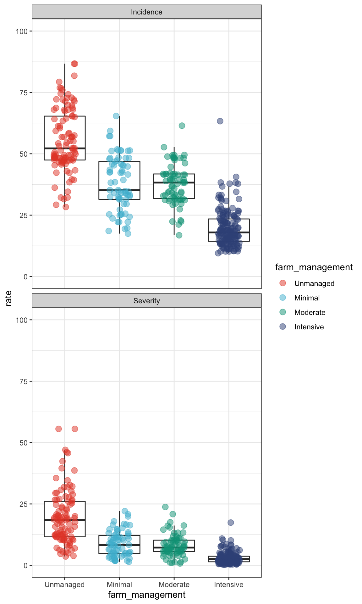
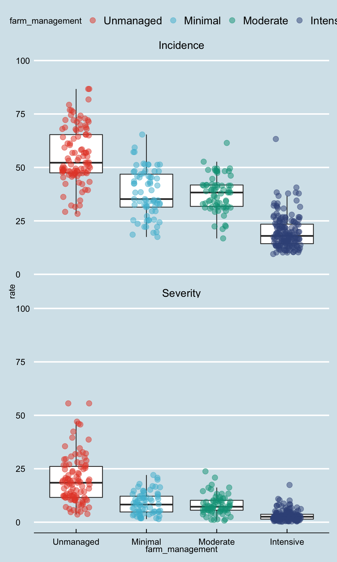
Here is the plot that we will eventually build today. We will show you the code first, and the finished product, but will walk through how to build this graph step-by-step.
ggplot(survey_data_long, aes(x= farm_management, y = rate))+

  geom_boxplot(outlier.alpha = 0)+
  geom_jitter(aes(color = farm_management),
              size = 3, width = 0.2, alpha = .5)+

  facet_wrap(~metric, ncol = 1)+
  scale_color_npg()+

  labs(title = "Disease distribution across farm management",
       x = NULL,
       y = "Percent (%)",
       color = "Farm management")+

  theme(
    panel.background = element_blank() ,
    panel.grid.major = element_line(colour = "grey88") ,
    panel.border     = element_rect(colour = "grey80", fill = NA) ,

    axis.text.y  = element_text(colour = "black"),
    axis.text.x  = element_blank(),
    title = element_text(face = "bold", size = 13),

    legend.position = c(0.70, .37),
    legend.key = element_rect(fill = "white"),
    legend.text = element_text(colour = "black", size=12),

    strip.text.x =  element_text(hjust =0.01, face = "bold", size = 14),
    strip.background =  element_blank())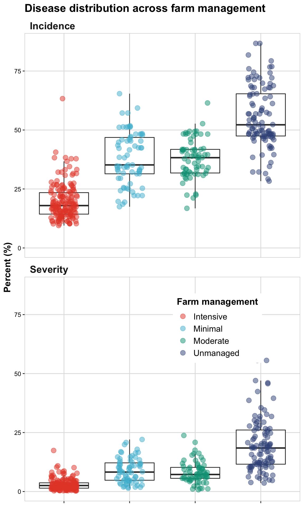
ggplot2 basics
Data organization
##
## ── Column specification ────────────────────────────────────────────────────────
## cols(
##   farm = col_double(),
##   region = col_character(),
##   zone = col_character(),
##   district = col_character(),
##   lon = col_double(),
##   lat = col_double(),
##   altitude = col_double(),
##   cultivar = col_character(),
##   shade = col_character(),
##   cropping_system = col_character(),
##   farm_management = col_character(),
##   inc = col_double(),
##   sev2 = col_double()
## )## # A tibble: 6 x 7
## altitude cultivar shade cropping_system farm_management inc sev2
## <dbl> <chr> <chr> <chr> <chr> <dbl> <dbl>
## 1 1100 Local Sun Plantation Unmanaged 86.7 55.6
## 2 1342 Mixture Mid shade Plantation Minimal 51.3 17.9
## 3 1434 Mixture Mid shade Plantation Minimal 43.2 8.25
## 4 1100 Local Sun Plantation Unmanaged 76.7 46.1
## 5 1400 Local Sun Plantation Unmanaged 47.2 12.3
## 6 1342 Mixture Mid shade Plantation Minimal 51.3 19.9Let’s get started with ggplot. What happens if we only run ggplot() without any additional information?

Not much! We need to be sure to specify the data (survey_data) and aesthetic elements (y and x axes).
## [1] "character"## NULLBUT- we still didn’t say anything about what type of plot we want.
Below we make sure that our data is in the correct form. For the graphs we would like to make, the farm management stratifies need to be set as factors.
survey_data = survey_data  %>%
  mutate(farm_management = factor(farm_management,
              levels = c("Unmanaged", "Minimal", "Moderate", "Intensive")))

head(survey_data)
## # A tibble: 6 x 7
## altitude cultivar shade cropping_system farm_management inc sev2
## <dbl> <chr> <chr> <chr> <fct> <dbl> <dbl>
## 1 1100 Local Sun Plantation Unmanaged 86.7 55.6
## 2 1342 Mixture Mid shade Plantation Minimal 51.3 17.9
## 3 1434 Mixture Mid shade Plantation Minimal 43.2 8.25
## 4 1100 Local Sun Plantation Unmanaged 76.7 46.1
## 5 1400 Local Sun Plantation Unmanaged 47.2 12.3
## 6 1342 Mixture Mid shade Plantation Minimal 51.3 19.9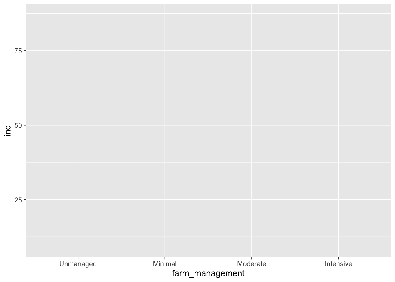
## [1] "factor"## [1] "Unmanaged" "Minimal" "Moderate" "Intensive"Now we can start adding the “meat and potatoes” to the graph.
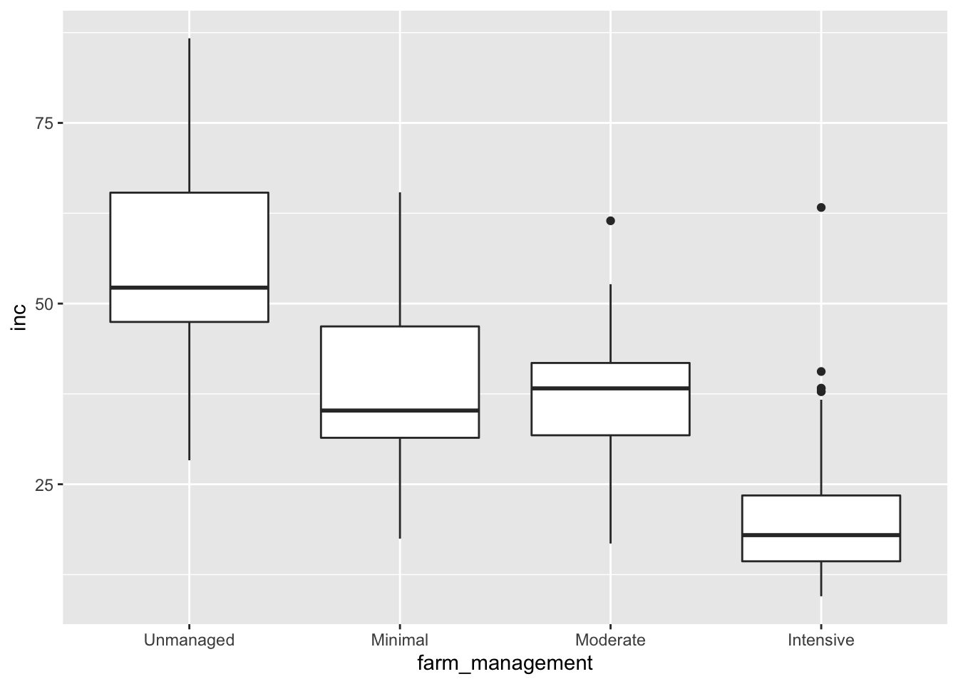
Here, we add the simple box plot geometry:
Alternatively, we can use the geom_point() geometry:
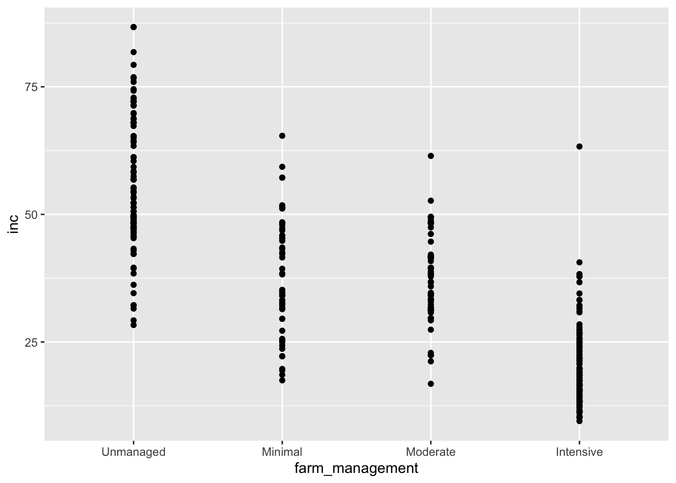
Well, it’s hard to see the individual points in the plot above, so lets “jitter” them from side to side with the jitter geometry:
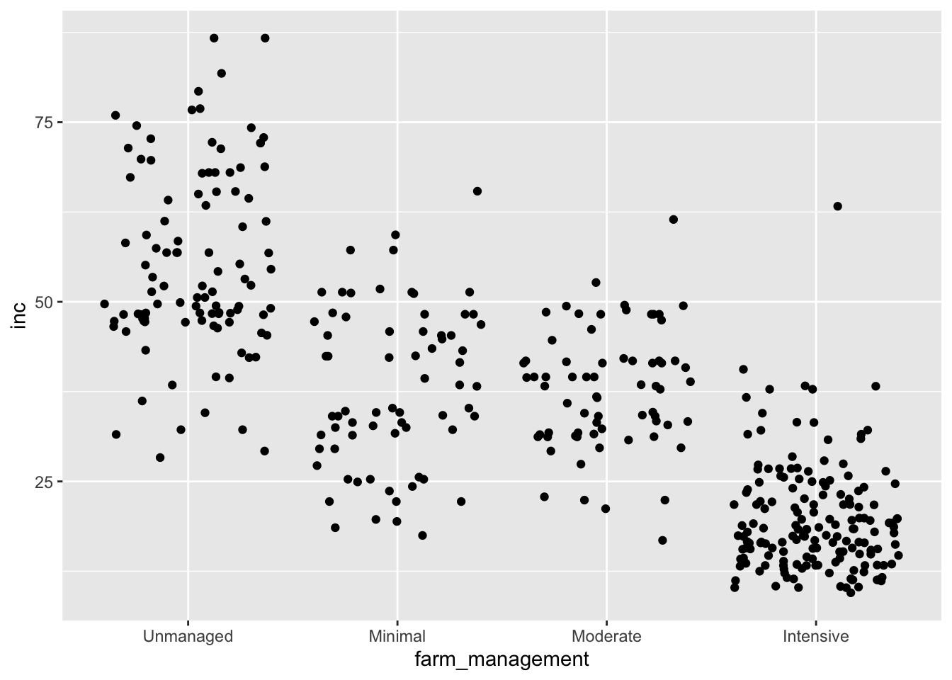
ggplot(survey_data, aes(x= farm_management, y = inc))+
geom_jitter(width = 0.2) # make the width a bit smaller 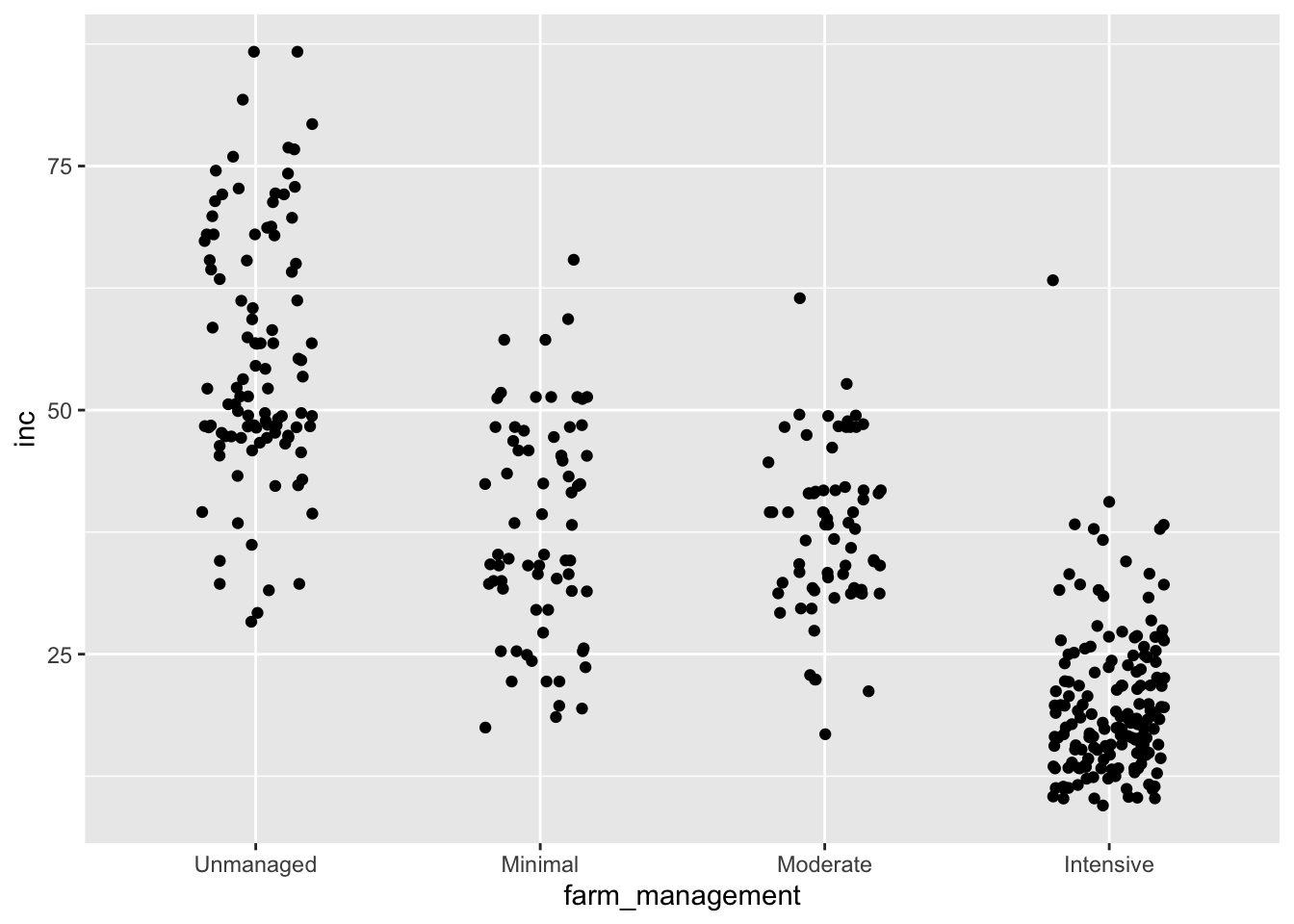
It would be even better if we could see both the data points AND the summary information that is available in a boxplot. Here we layer two geometries: geom_jitter and geom_boxplot.
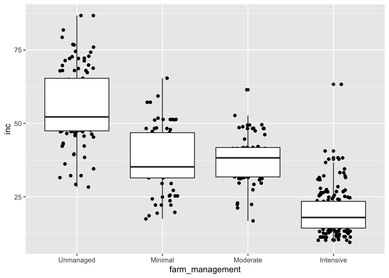
See what happens when you reverse the order of those geometries:
ggplot(survey_data, aes(x= farm_management, y = inc))+
geom_boxplot(outlier.alpha = 0) +
geom_jitter(width = 0.2)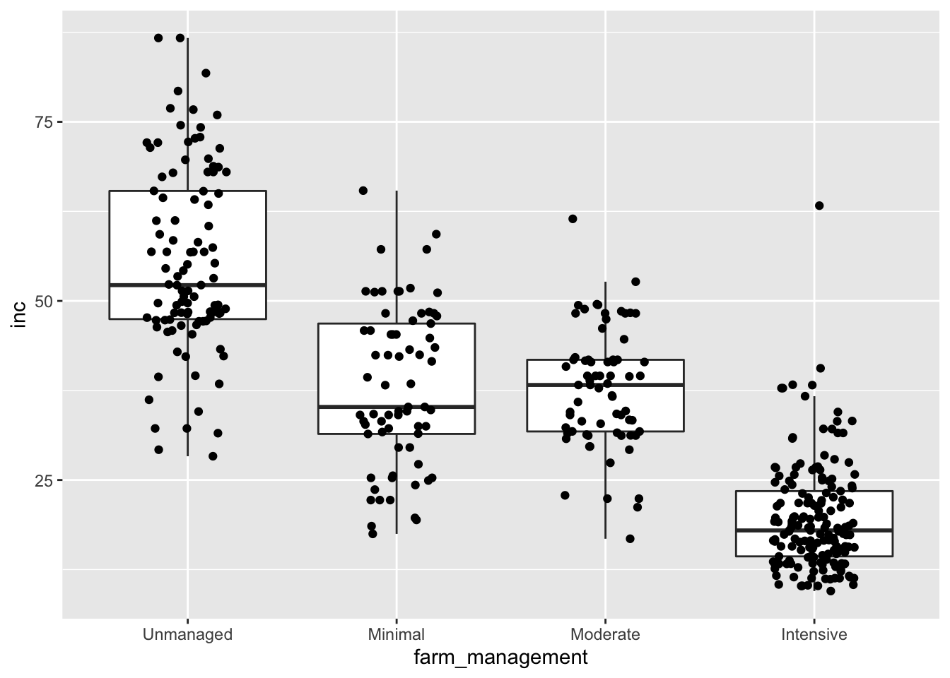
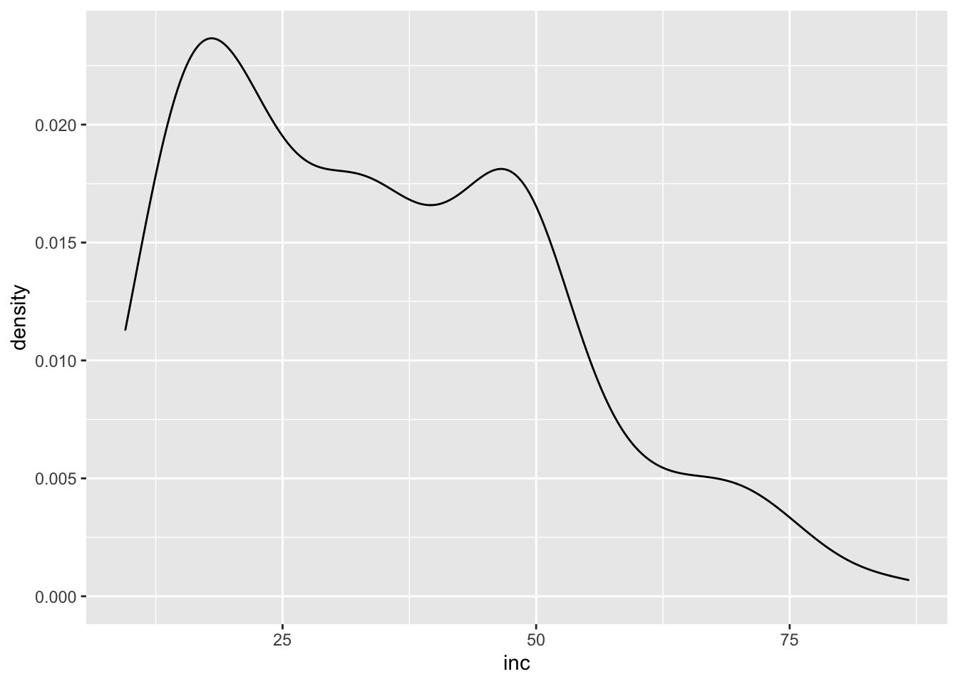
Some other useful geometries include geom_violin, geom_histogram, and geom_density. These each give information about the distribution of our data:
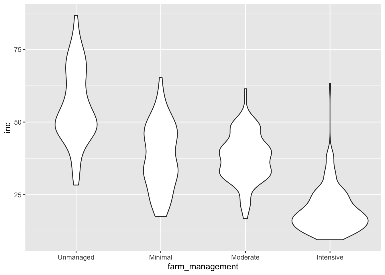
## `stat_bin()` using `bins = 30`. Pick better value with `binwidth`.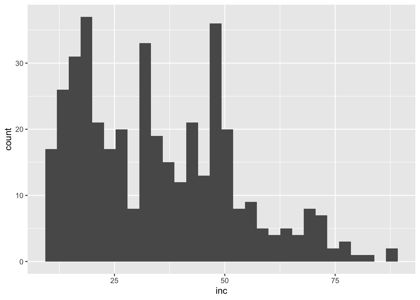
Here we look at geom_dotplot and geom_point(). Adding geom_smooth() and geom_rug() to geom_point() allow you to present additional information about the smoothed mean and distribution of data points.
ggplot(survey_data,aes(x= farm_management, y = inc))+
geom_dotplot(binaxis = "y",
stackdir = "center", binwidth = 1.2)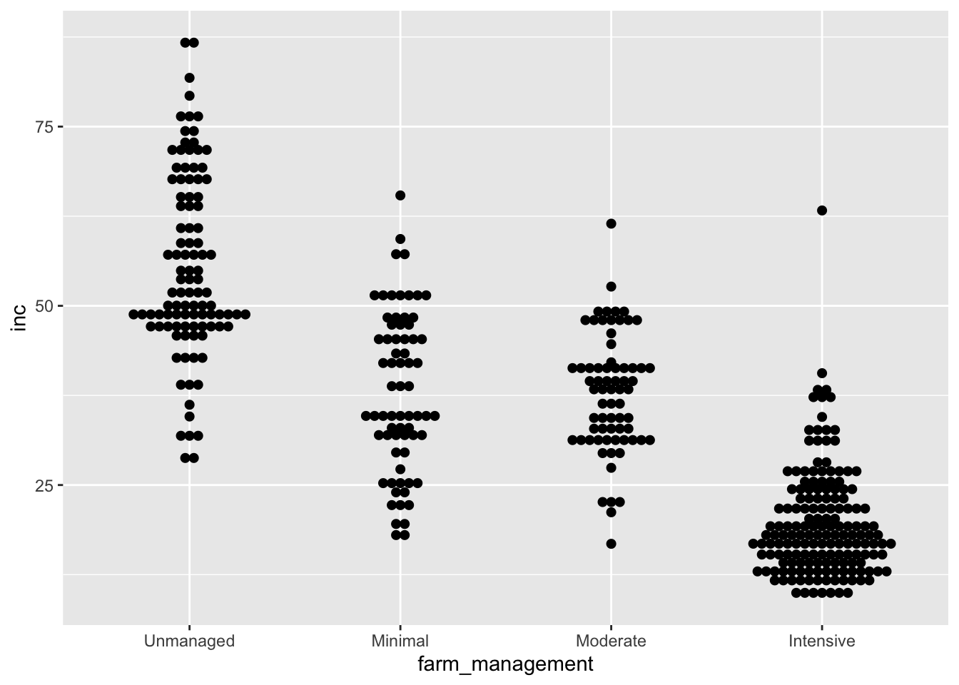
## `geom_smooth()` using method = 'loess' and formula 'y ~ x'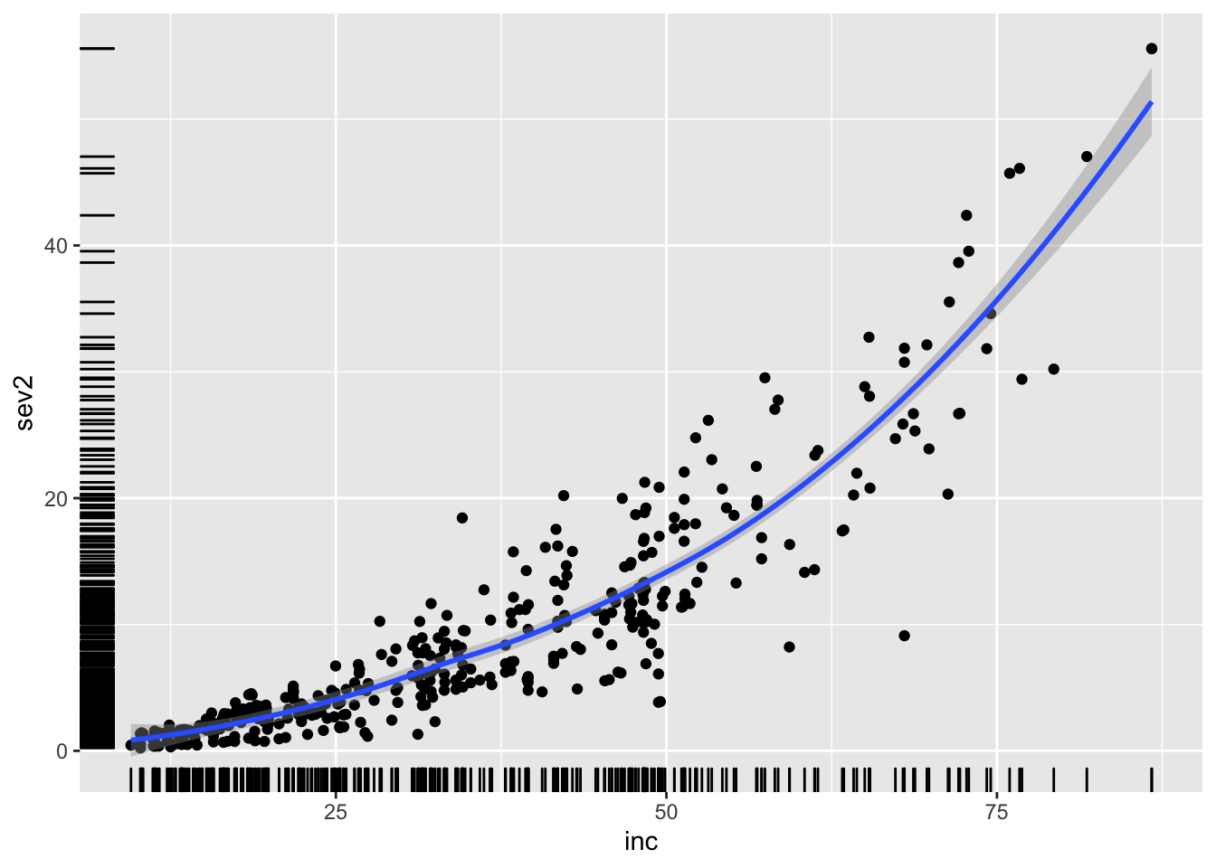
Aesthetics
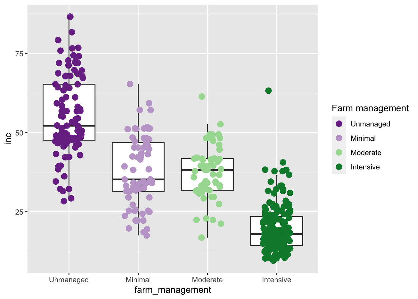
Choosing aesthetics is critical for communicating the message of a plot. Colors, for example can be used strategically to convey information. Here we color by farm management type:
ggplot(survey_data, aes(x= farm_management, y = inc,
shape = farm_management,
color = farm_management))+
geom_boxplot(outlier.alpha = 0) +
geom_jitter(width = 0.2)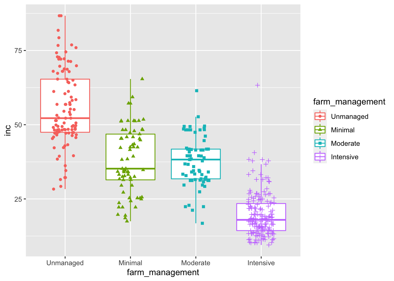
ggplot(survey_data, aes(x= farm_management, y = inc))+
geom_boxplot(outlier.alpha = 0) +
geom_jitter(aes(color = farm_management),width = 0.2)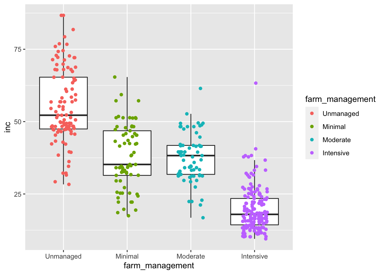
We can change the size of points as well as the transparency.
ggplot(survey_data, aes(x= farm_management, y = inc))+
geom_boxplot(outlier.alpha = 0) +
geom_jitter(aes(color = farm_management),width = 0.2,
size = 3)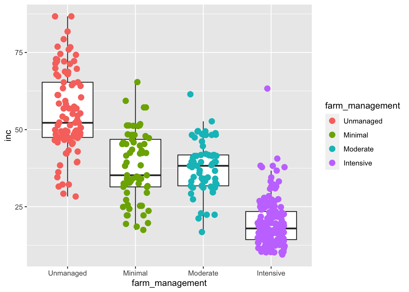
ggplot(survey_data, aes(x= farm_management, y = inc))+
geom_boxplot(outlier.alpha = 0) +
geom_jitter(aes(colour = farm_management),width = 0.2,
size = 3, alpha = 0.5)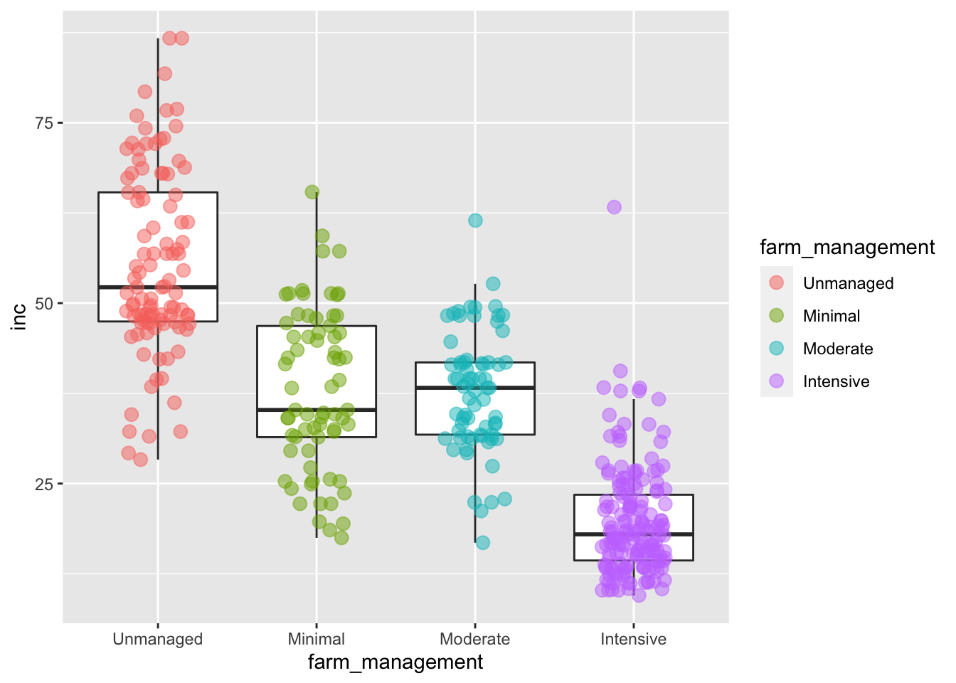
‘fill’ will apply color to the variable you indicate:
ggplot(survey_data, aes(x= farm_management, y = inc))+
geom_jitter(width = 0.2, size = 4, shape = 21,
aes(fill = altitude ))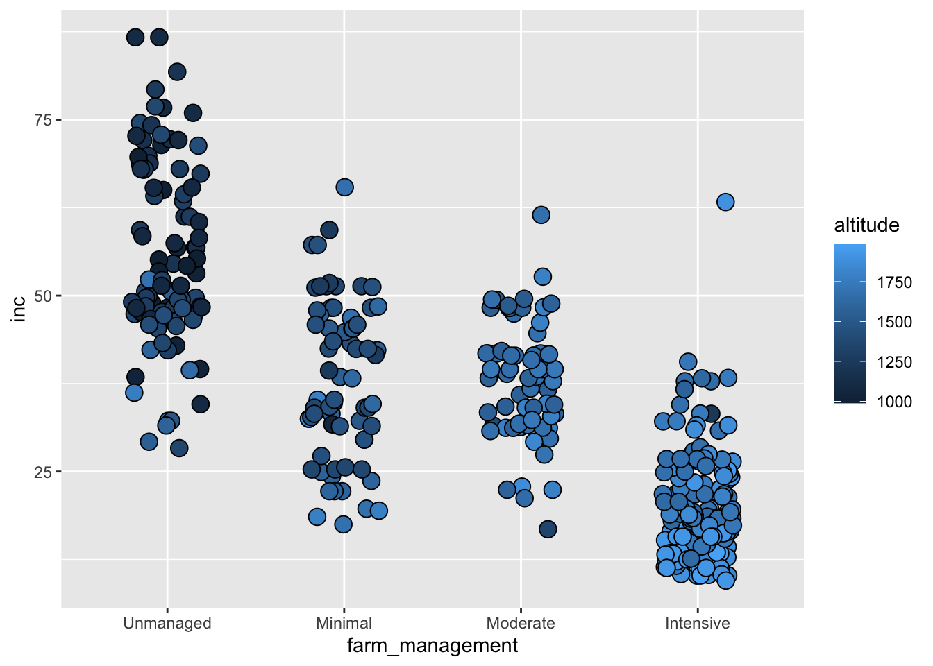
Size of points as well as transparency can be changed by setting ‘size’ or ‘alpha’ equal to the continuous variable that you would like to use.
ggplot(survey_data, aes(x= farm_management, y = inc))+
geom_jitter(width = 0.2, size = 4,
aes(alpha = sev2 ))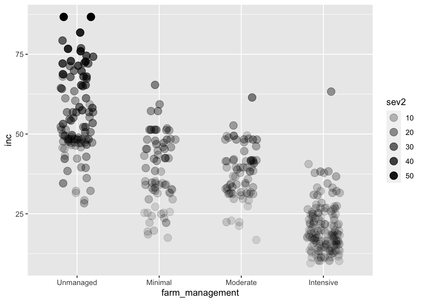
ggplot(survey_data, aes(x= farm_management, y = inc))+
geom_jitter(width = 0.2, shape = 21, fill = "grey",
aes(size = sev2 ))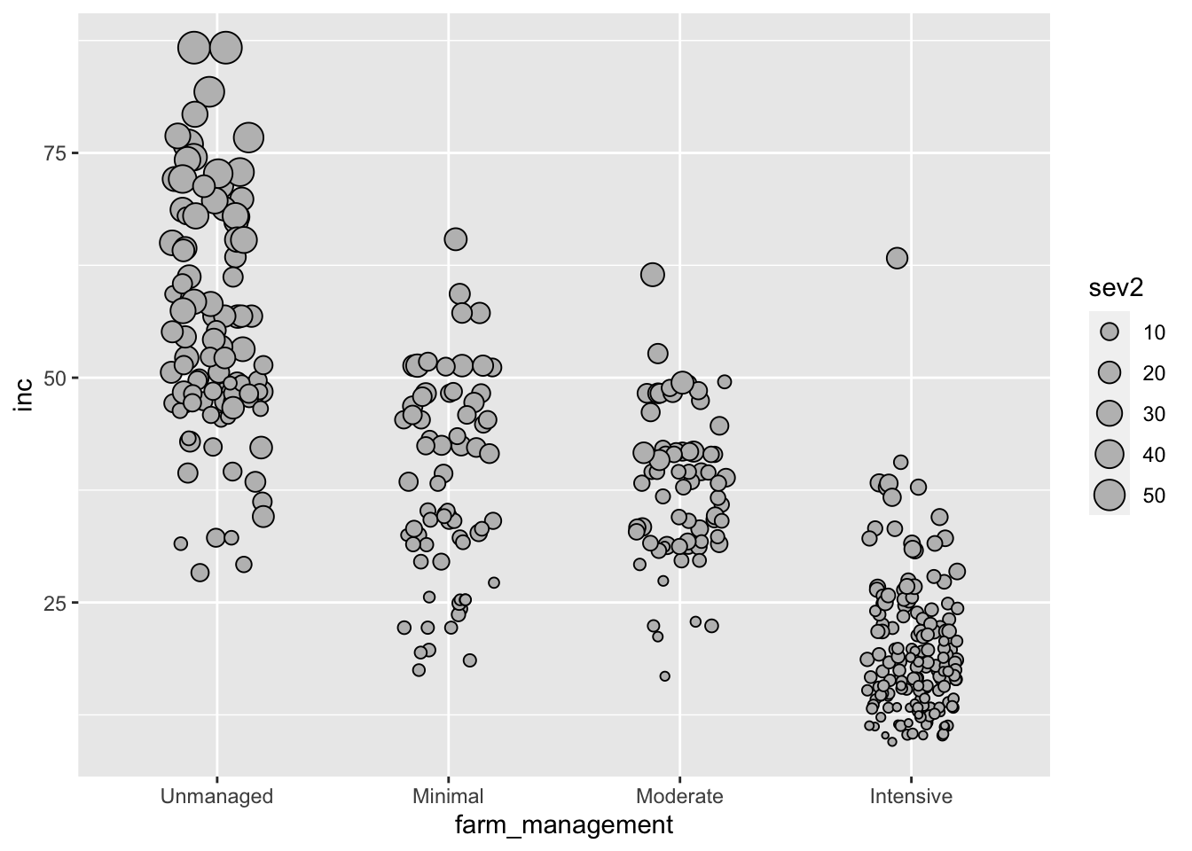
Change the shapes of each level (a good option if a figure will be black and white).
ggplot(survey_data, aes(x= farm_management, y = inc))+
geom_jitter(width = 0.2, size = 3, alpha = 0.8,
aes(shape = farm_management))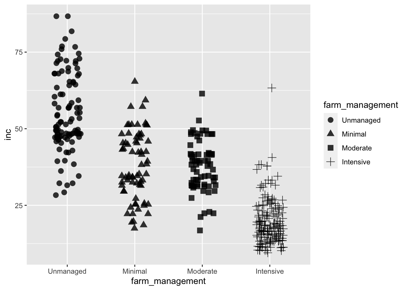
You can also adjust the border color of points:
ggplot(survey_data, aes(x= farm_management, y = inc))+
geom_jitter(width = 0.2, size = 3, alpha = 0.8, shape = 21,
aes(color = farm_management))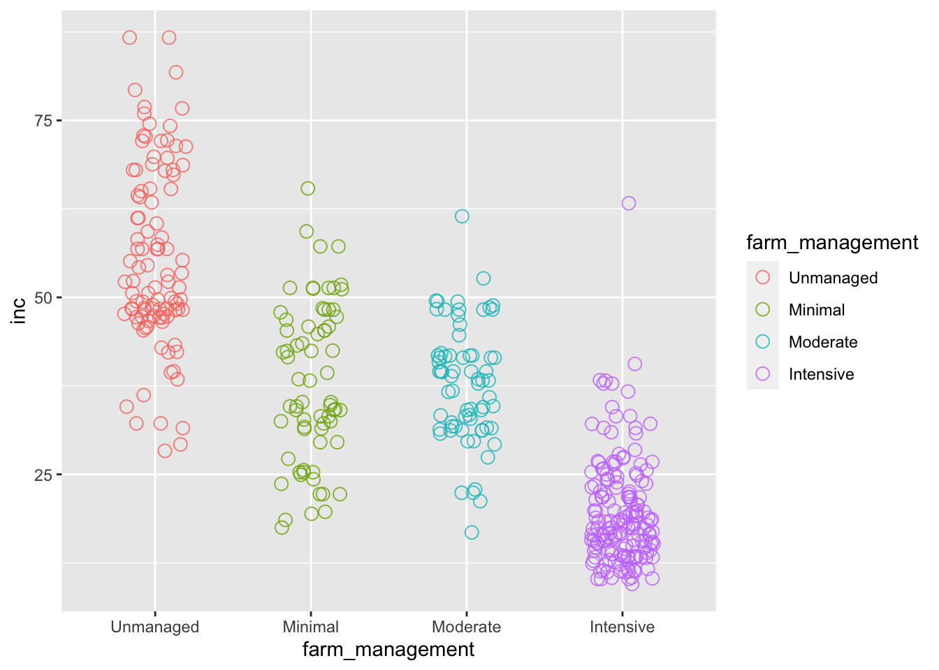
ggplot(survey_data, aes(x= farm_management, y = inc))+
geom_jitter(width = 0.2, size = 3, alpha = 0.8, shape = 21,
aes(fill = farm_management))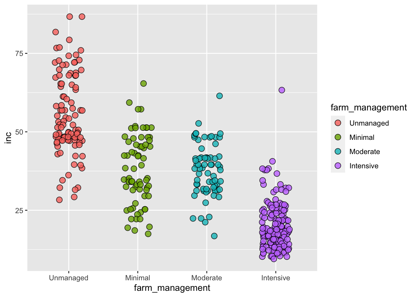
## `geom_smooth()` using method = 'loess' and formula 'y ~ x'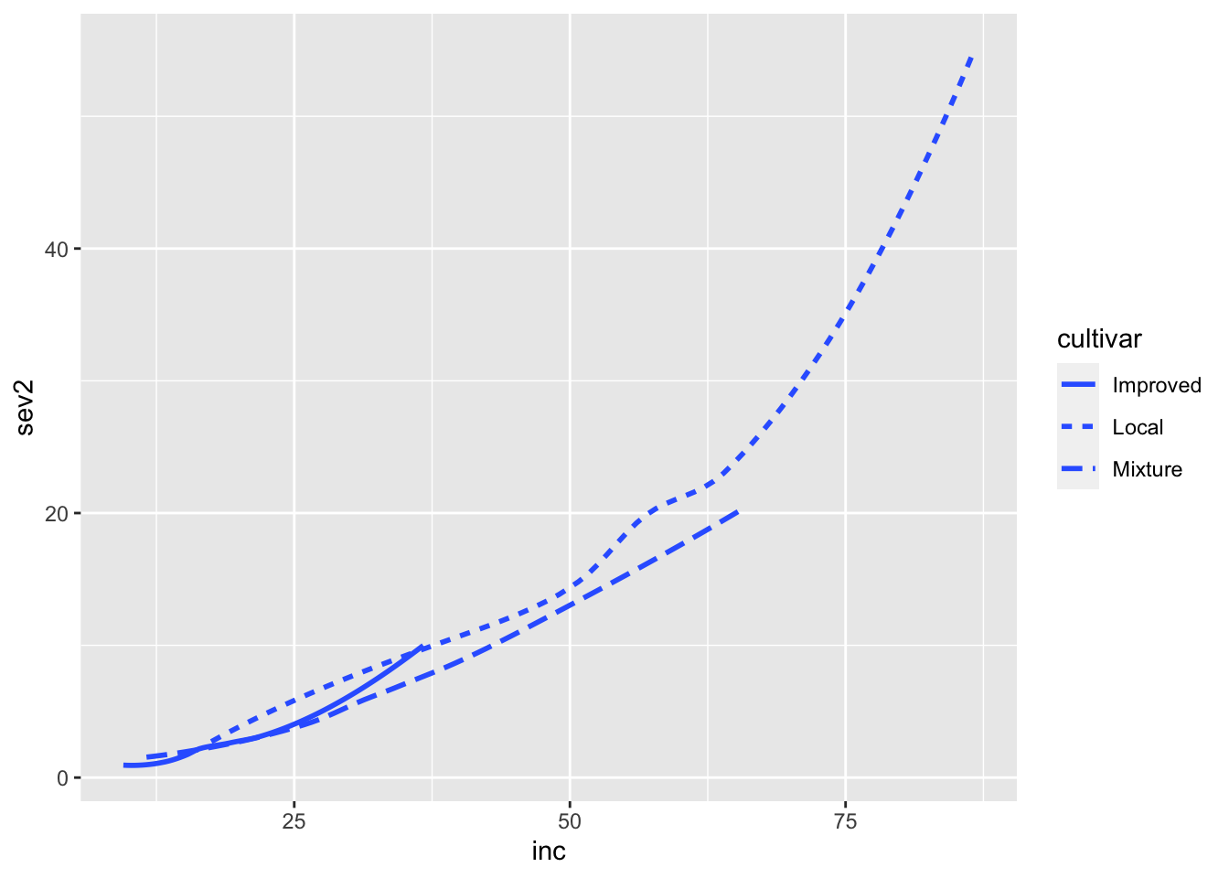
ggplot(survey_data, aes(x=inc , y = sev2, color = cultivar))+
geom_point(alpha = 0.2)+
geom_smooth(aes(linetype = cultivar), se = FALSE)+
geom_rug()## `geom_smooth()` using method = 'loess' and formula 'y ~ x'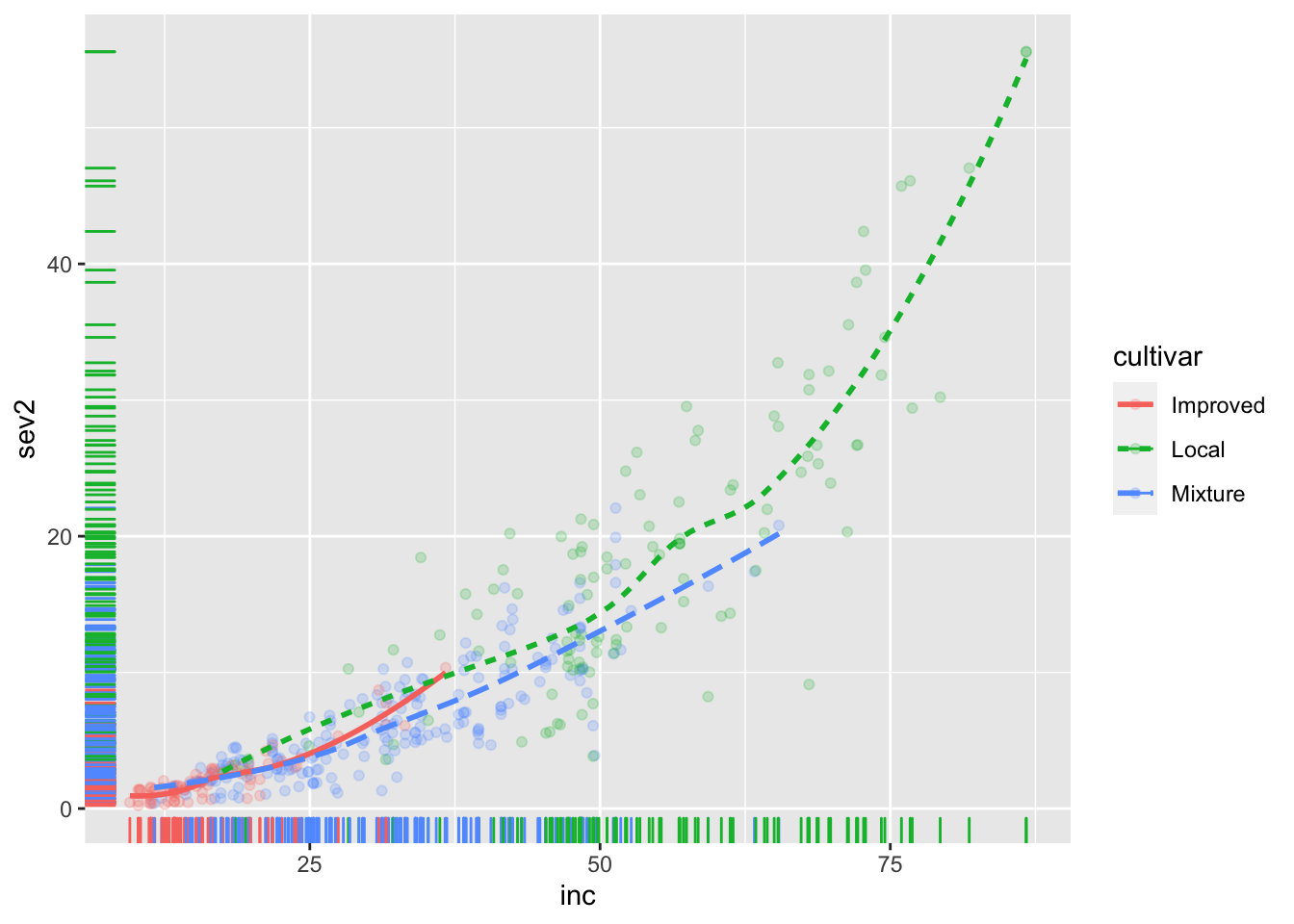
Scales
You can manually adjust the x and y axis scales. This can be very useful when creating publication ready plots.
p = ggplot(survey_data, aes(x= farm_management, y = inc))+
geom_boxplot(outlier.alpha = 0) +
geom_jitter(aes(colour = farm_management),
width = 0.2,size = 3)
p + scale_y_continuous(name = "Incidence (%)",
breaks = c(0,25,50, 75, 100),
limits = c(0,100))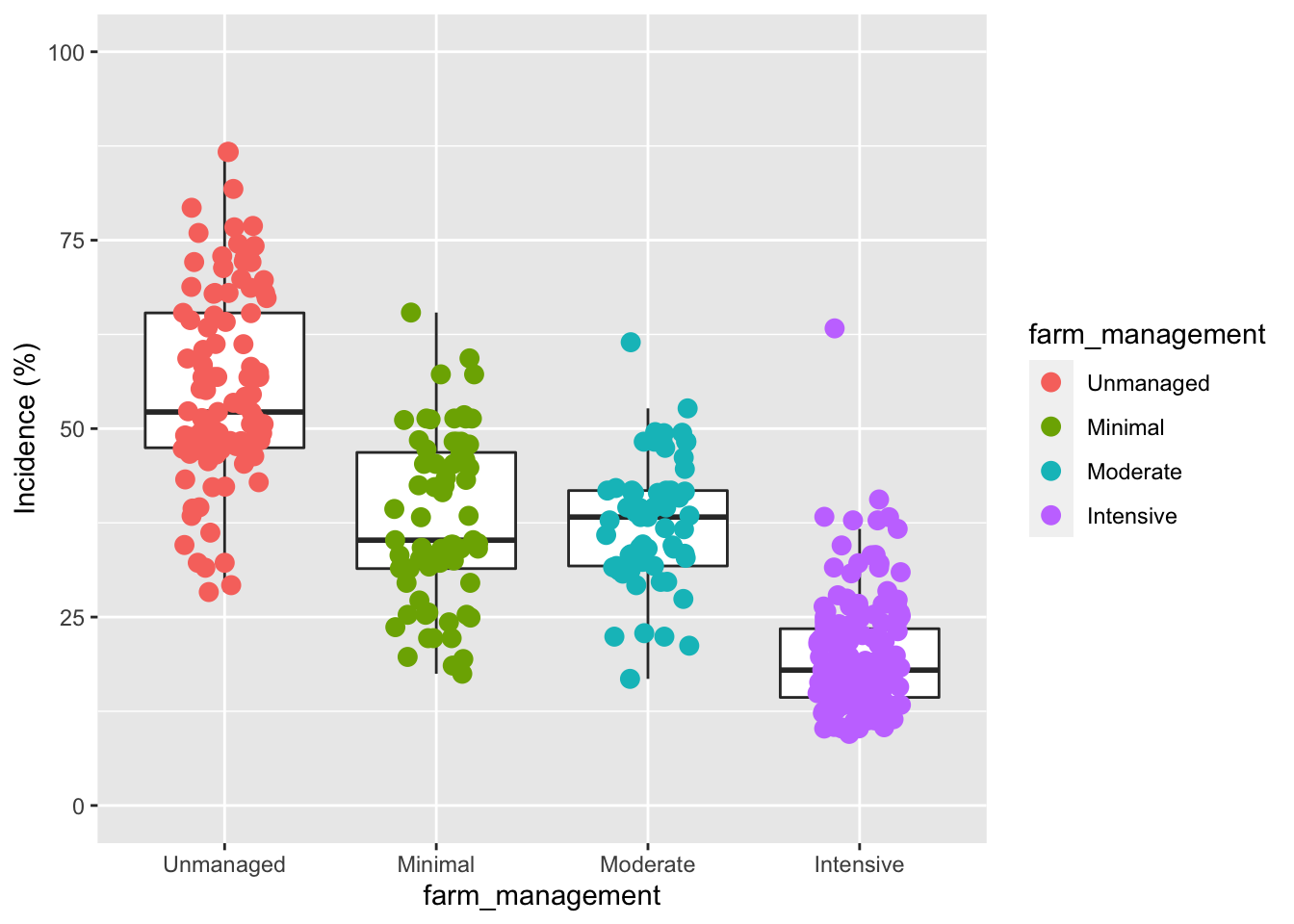
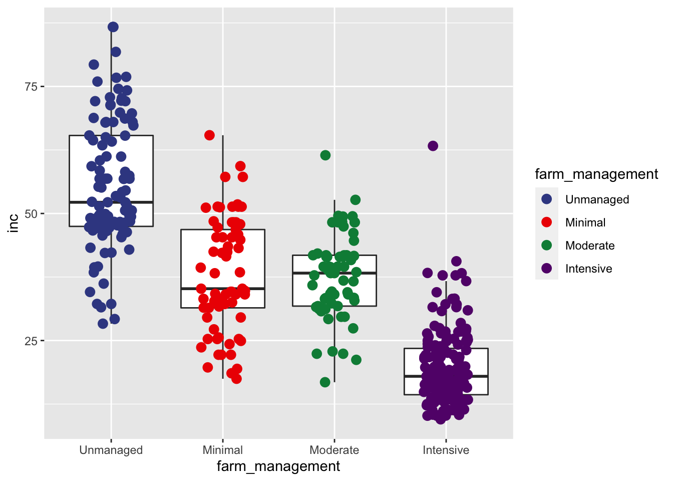
You can also manually change the colors of factor levels.
p + scale_color_manual(
name = "Farm management",
values = c("blue", "grey80", "#2ca25f", "#756bb120"))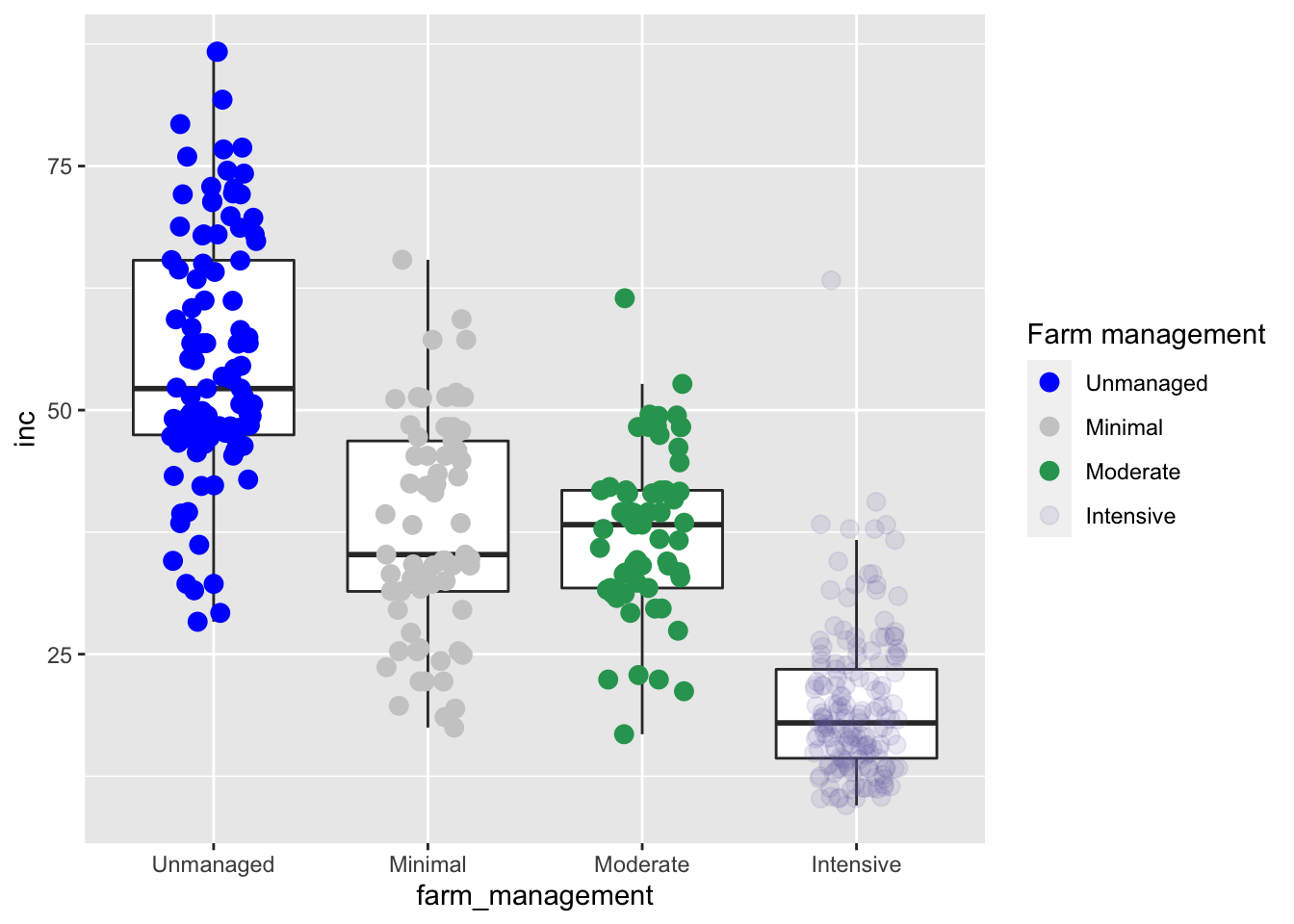
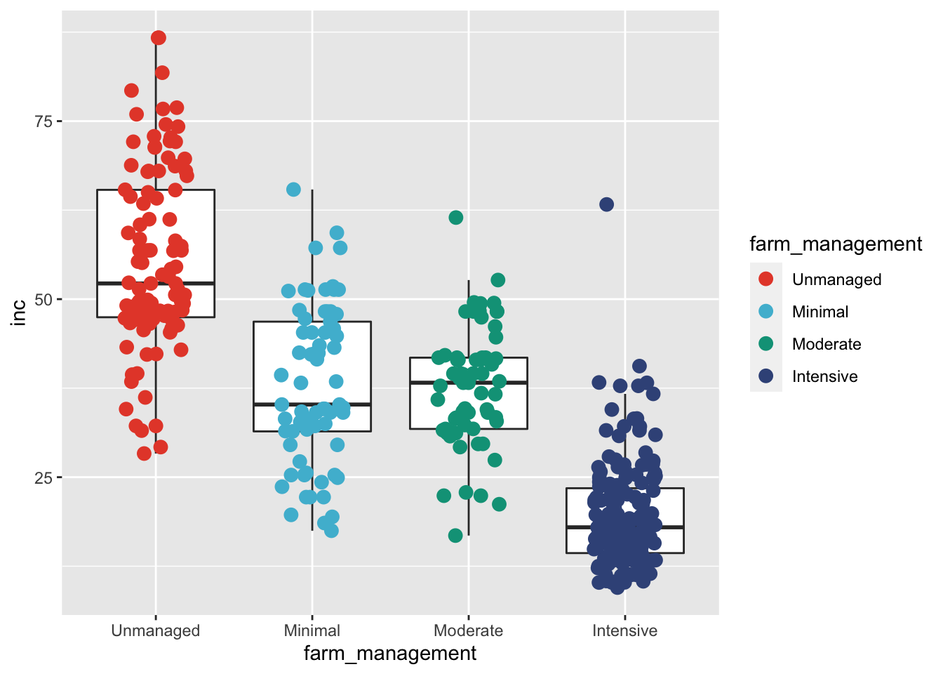
There are pre-defined color palettes in scale_color_brewer:
ggsci is a package that offers a collection of color palettes inspired by colors used in scientific journals, data visualization libraries, science fiction movies, and TV shows.
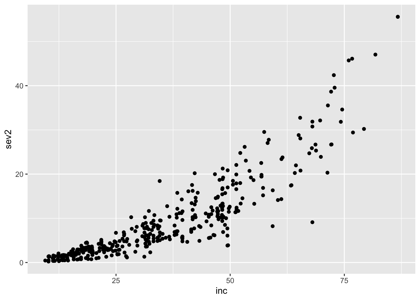
Lines can also be changed in ggplot, here is an example where we manually changed the type of line for each level. This graph shows incidence vs. severity.
ggplot(survey_data, aes(x=inc , y = sev2))+
geom_smooth(se = FALSE, aes(linetype = cultivar, color = cultivar))+
# scale_linetype_manual(values = c(1,2,4)) +
scale_linetype_manual(values = c("solid","longdash", "991191"))## `geom_smooth()` using method = 'loess' and formula 'y ~ x'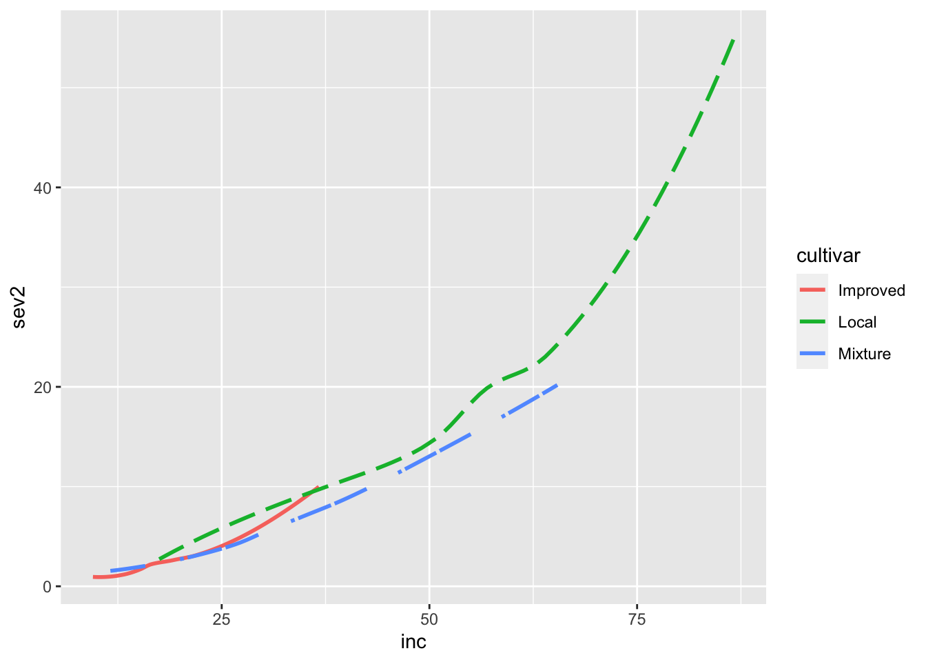
Facets
Faceting is an easy way to break data into multipe plots with the same themes.
## # A tibble: 6 x 7
##   altitude cultivar shade     cropping_system farm_management   inc  sev2
##      <dbl> <chr>    <chr>     <chr>           <fct>           <dbl> <dbl>
## 1     1100 Local    Sun       Plantation      Unmanaged        86.7 55.6
## 2     1342 Mixture  Mid shade Plantation      Minimal          51.3 17.9
## 3     1434 Mixture  Mid shade Plantation      Minimal          43.2  8.25
## 4     1100 Local    Sun       Plantation      Unmanaged        76.7 46.1
## 5     1400 Local    Sun       Plantation      Unmanaged        47.2 12.3
## 6 1342 Mixture Mid shade Plantation Minimal 51.3 19.9Here we need to make sure our data is correctly organized. This will help us visualize incicence and severity side-by-side. We also rename inc to “Incidence” and sev2 to “Severity” because these will be the labels of our facet plots.
survey_data_long = survey_data  %>%
   pivot_longer(cols = c(inc, sev2),
               names_to = "metric",
               values_to = "rate") %>%

   mutate(metric = factor(metric,
                         levels = c("inc", "sev2"),
                         labels = c("Incidence", "Severity")))

head(survey_data_long)
## # A tibble: 6 x 7
## altitude cultivar shade cropping_system farm_management metric rate
## <dbl> <chr> <chr> <chr> <fct> <fct> <dbl>
## 1 1100 Local Sun Plantation Unmanaged Incidence 86.7
## 2 1100 Local Sun Plantation Unmanaged Severity 55.6
## 3 1342 Mixture Mid shade Plantation Minimal Incidence 51.3
## 4 1342 Mixture Mid shade Plantation Minimal Severity 17.9
## 5 1434 Mixture Mid shade Plantation Minimal Incidence 43.2
## 6 1434 Mixture Mid shade Plantation Minimal Severity 8.25Save plot as ‘p2’ and plot ‘p2’.
p2 = ggplot(survey_data_long, aes(x= farm_management, y = rate))+
geom_boxplot(outlier.alpha = 0)+
geom_jitter(aes(color = farm_management),
size = 3, width = 0.2, alpha = .5)+
scale_y_continuous(breaks = seq(0,100,25),
limits = c(0,100))+
scale_color_npg()
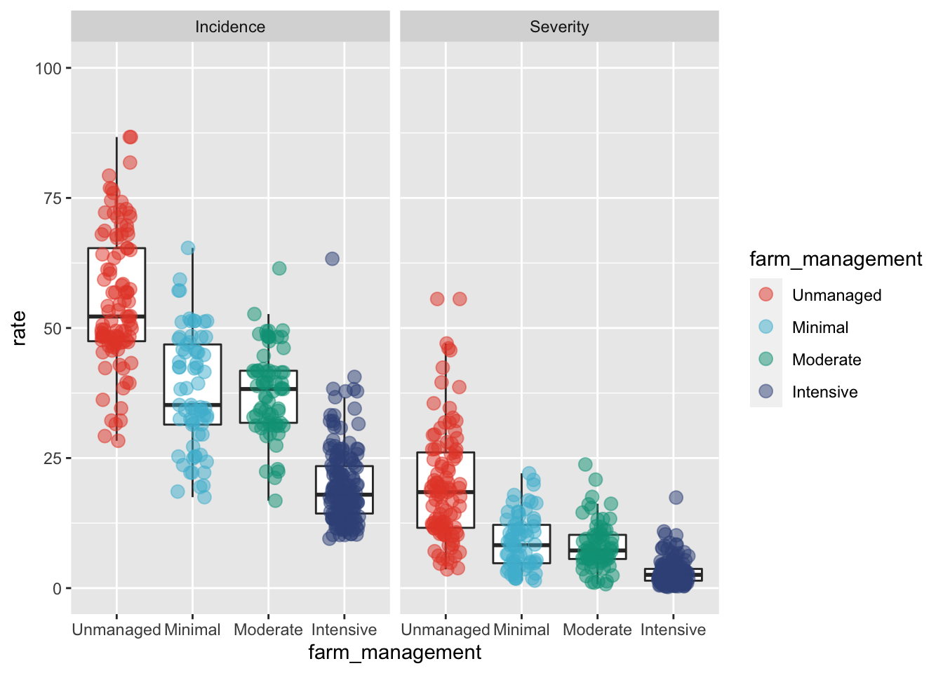
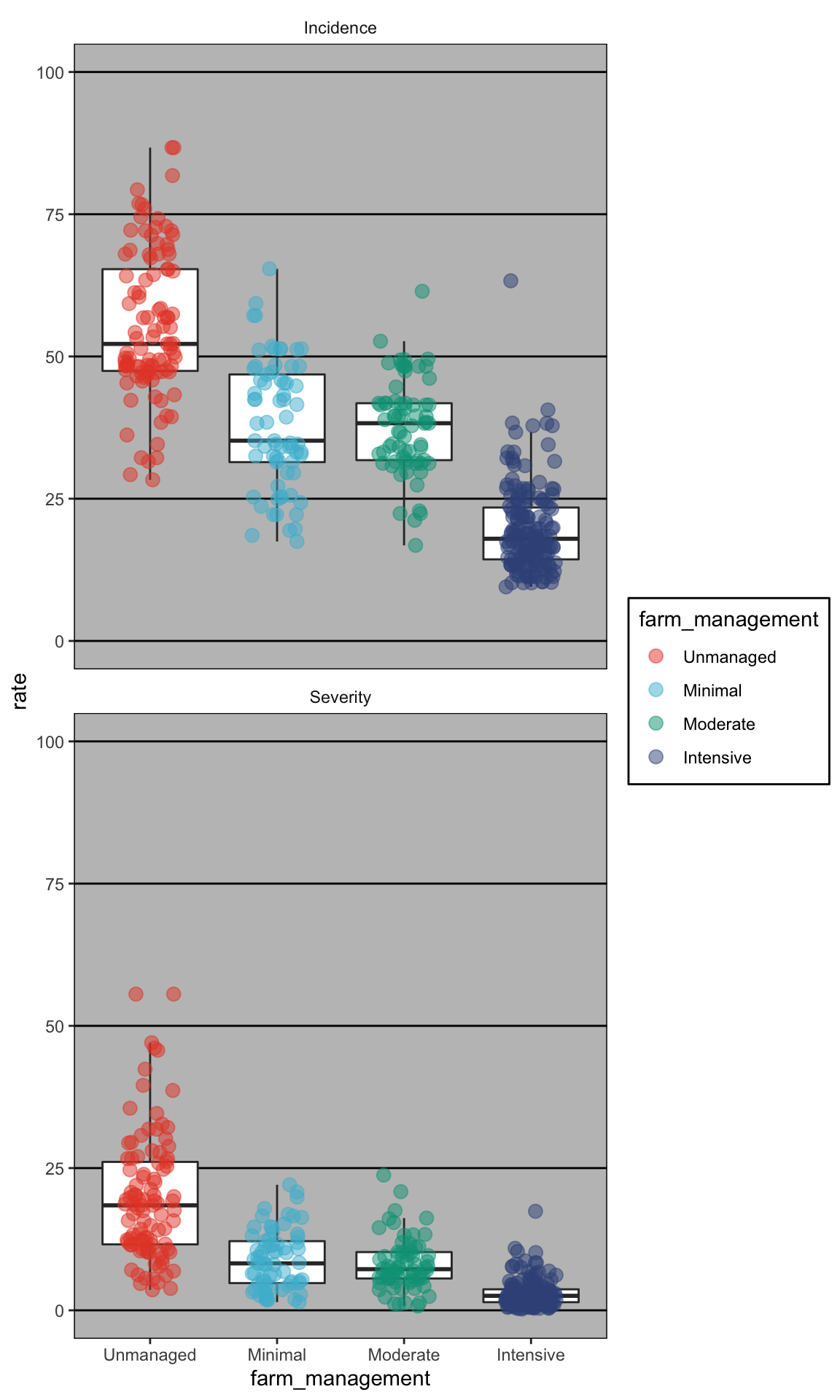
p2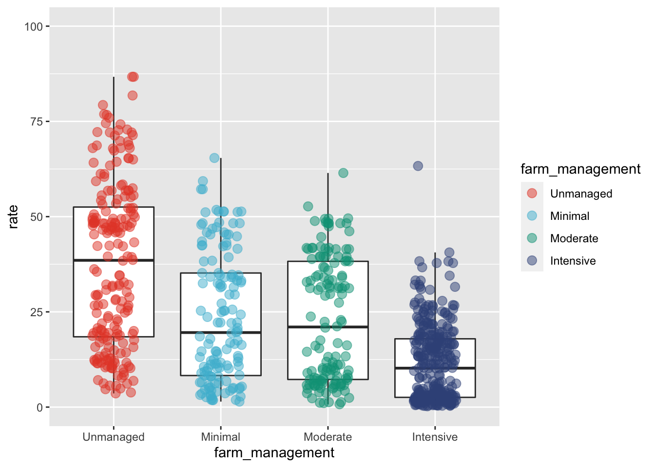 Here we facet_wrap by metric (incidence and severity are our metrics):
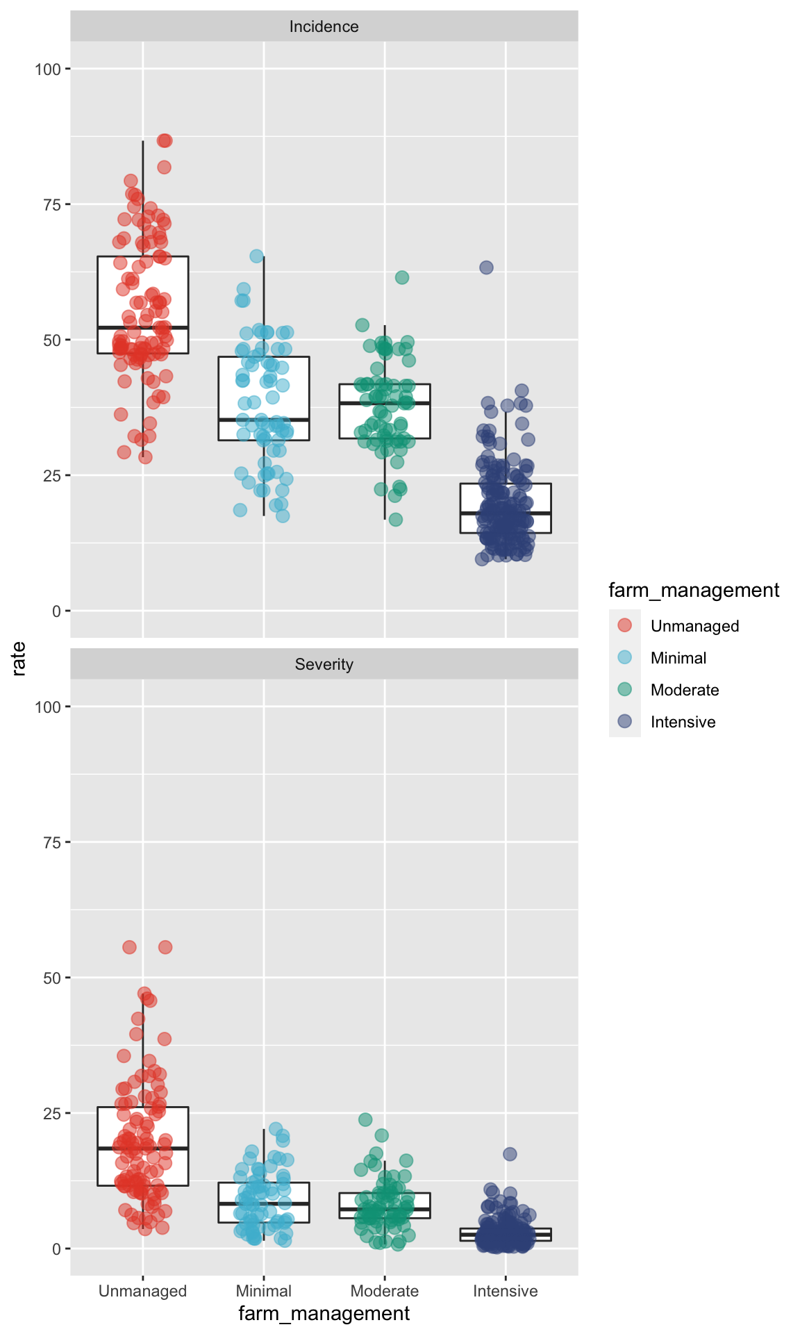
If we specify the number of columns (ncol) as 1, the plots will be stacked into a single column.
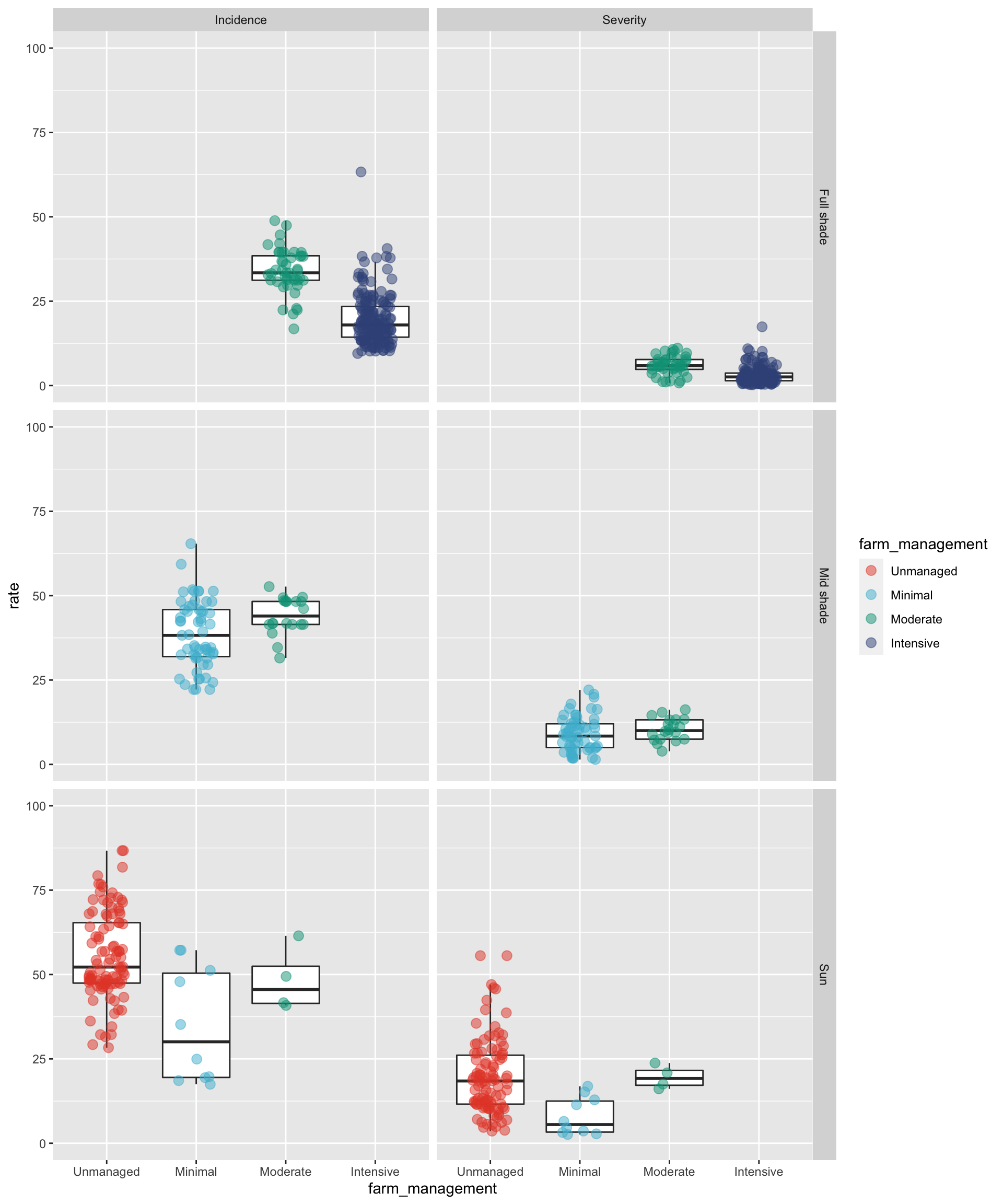
facet_grid() allows us to create a grid of plots.
Labels
Here we can add custom titles, subtitles, and footnotes.
  p2 + facet_wrap(~metric, ncol = 1)+

  labs(title = "Plot title",
       subtitle = "Here is a subtitle",
       x = NULL, # suppress x-axis title
       y = "y-axis title",
       color = "Legend title",
       caption = "Hey!!! This can be a footnote")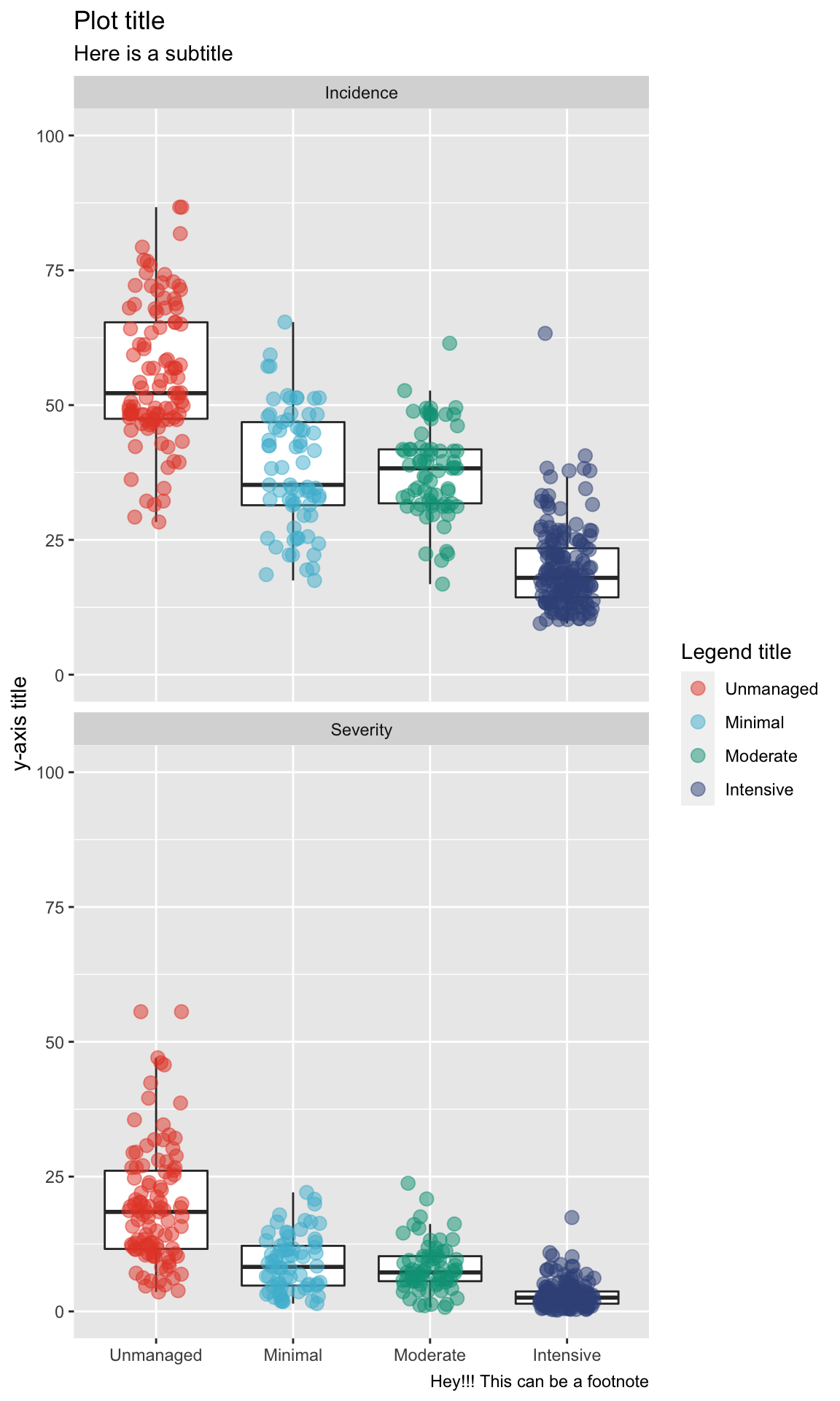
Themes
Themes are pre-defined themes that are built into ggplot and can be slightly modified.
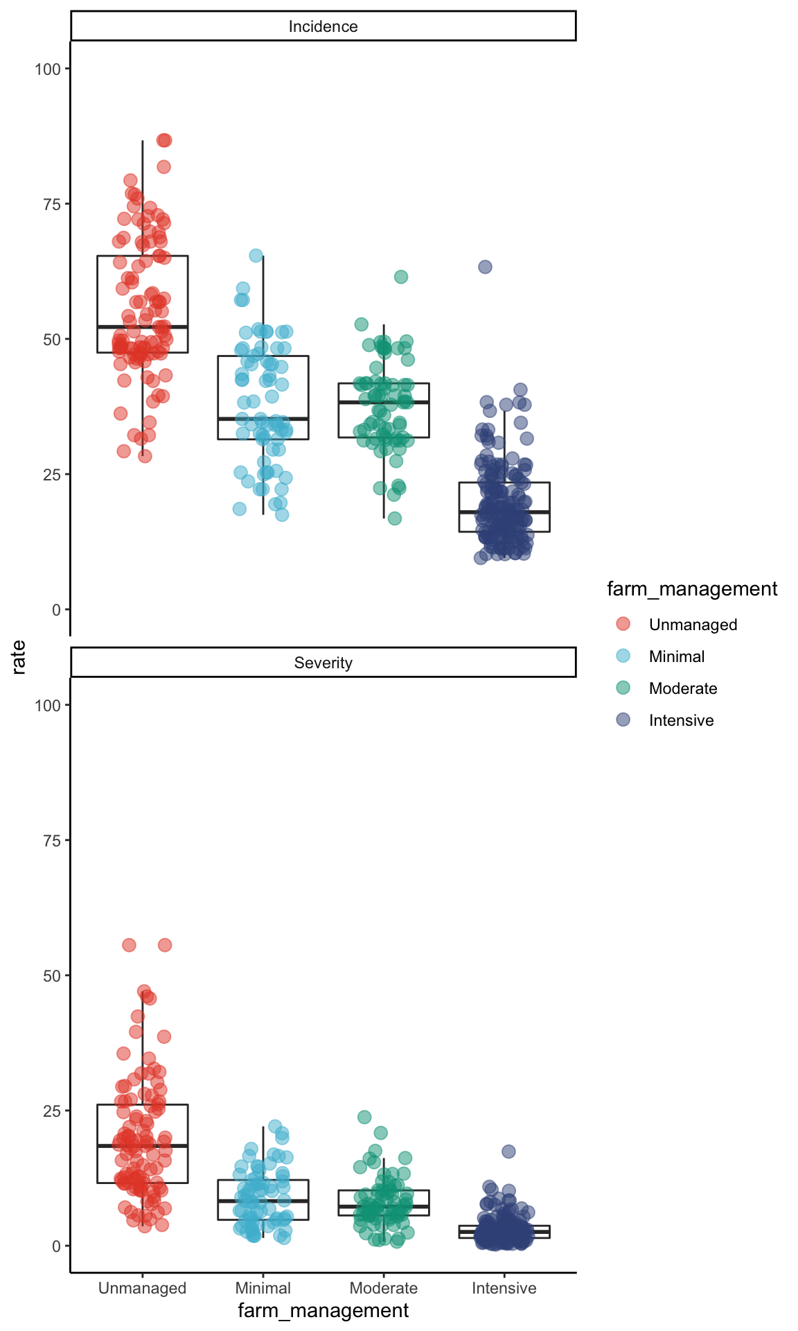
Here is theme classic:
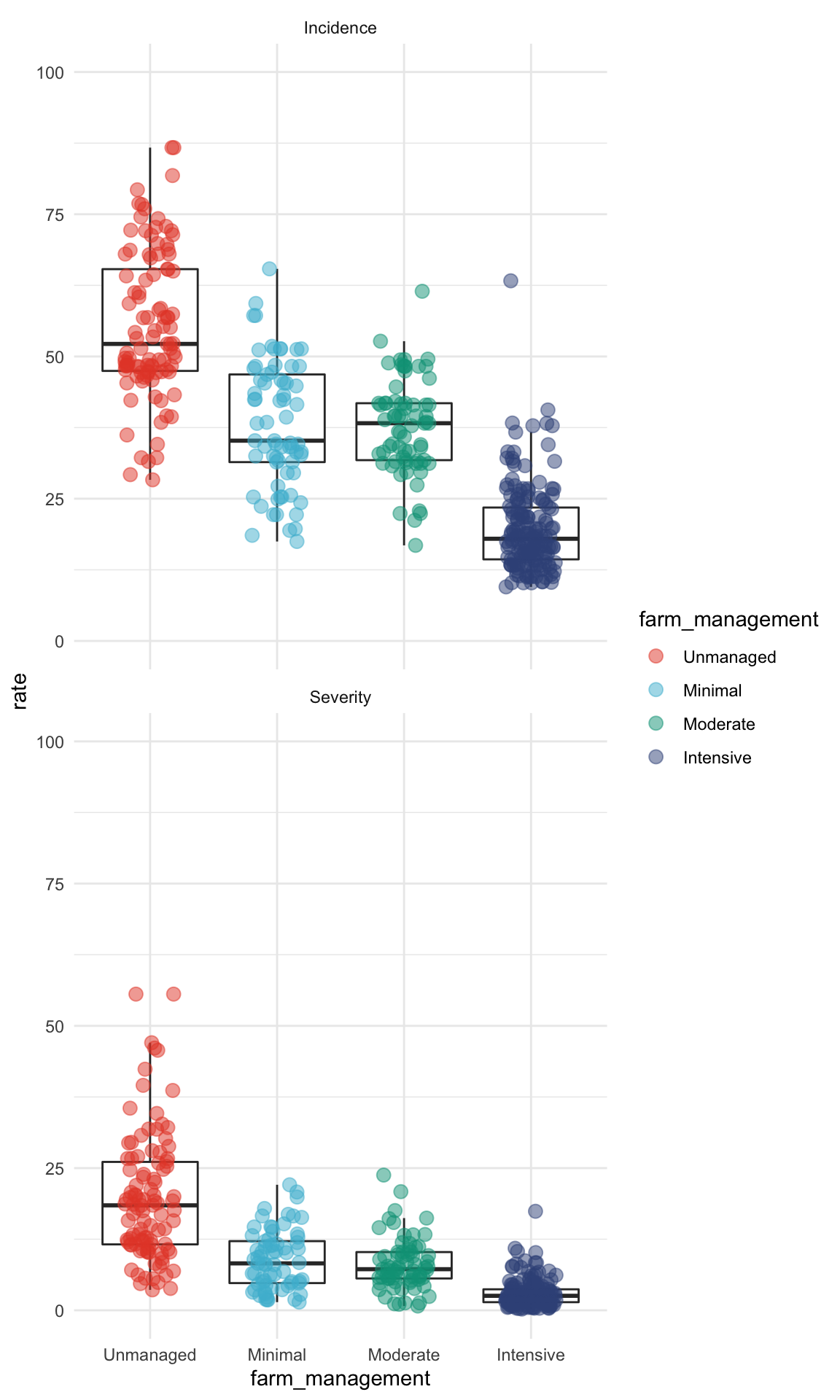
Here is theme minimal:
Here is theme Economist and theme Excel.
We can individually edit components of a theme. This can be particularly useful for making graphs for publications.
  p2 + facet_wrap(~metric, ncol = 1)+
  labs(x = NULL, y = "Percent (%)", color = "Farm Management")+

  theme(
    panel.background = element_blank() ,
    panel.grid.major = element_line(colour = "grey88") ,
    panel.border     = element_rect(colour = "grey80", fill = NA),

    axis.text.y  = element_text(colour = "black"),
    axis.text.x  = element_blank(),
    title = element_text(colour = "black", size = 12, face = "bold"),

    legend.position = c(0.85, .39),
    legend.key = element_rect(fill = "white"),
    legend.text = element_text(colour = "black", size = 12),

    strip.text.x =  element_text(hjust =0.01, face = "bold", size = 14),
    strip.background =  element_blank())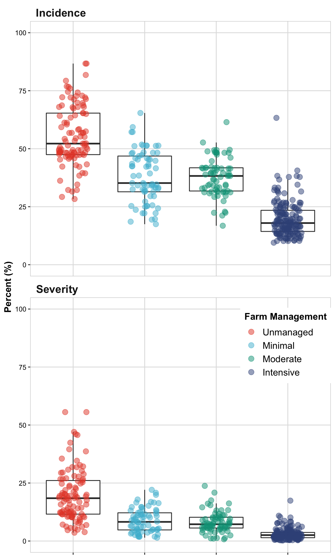
Save
Saving according to the size that you would like can be tricky, we recommend using ggsave.
 p3 =  p2 + facet_wrap(~metric, ncol = 1)+
      labs(x = NULL, y = "Percent (%)", color = "Farm Management")+

    theme(
      panel.background = element_blank() ,
      panel.grid.major = element_line(colour = "grey88") ,
      panel.border     = element_rect(colour = "grey80", fill = NA),

      axis.text.y  = element_text(colour = "black"),
      axis.text.x  = element_blank(),
      title = element_text(colour = "black", face = "bold"),

      legend.position = c(0.72, .33),
      legend.key = element_rect(fill = "white"),
      legend.text = element_text(colour = "black"),

      strip.text.x =  element_text(hjust =0.01, face = "bold"),
      strip.background =  element_blank())

   ggsave(plot = p3, filename = "graph/APS_plot_2.tiff",
         width =85, height = 140, units = "mm",
         dpi = 300)
   p3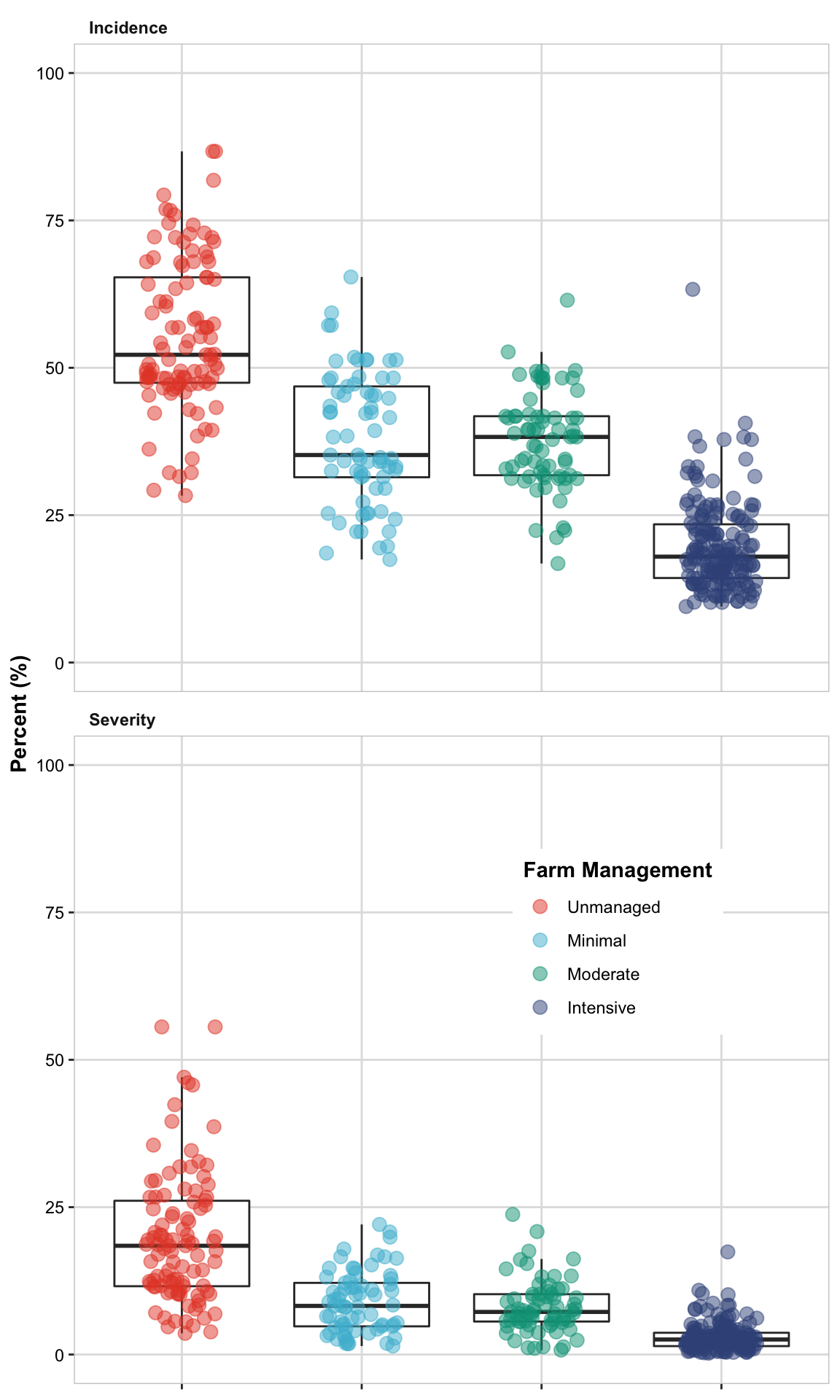
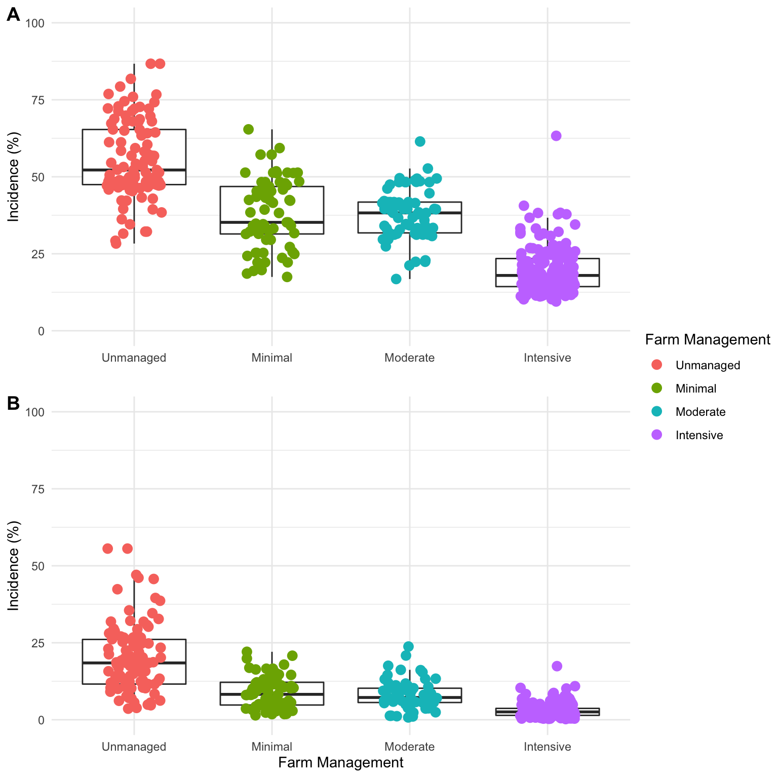
p4 =
ggplot(survey_data_long, aes(x= farm_management, y = rate))+
geom_boxplot(outlier.alpha = 0)+
geom_jitter(aes(color = farm_management),
size = 1.5, width = 0.3, alpha = .5)+
scale_y_continuous(breaks = seq(0,100,25),
limits = c(0,100))+
scale_color_npg()+
facet_wrap(~metric, ncol = 1)+
labs(x = NULL, y = "Percent (%)")+
theme(
panel.background = element_blank() ,
panel.grid.major = element_line(colour = "grey88") ,
panel.border = element_rect(colour = "grey80", fill = NA),
axis.text = element_text(colour = "black"),
title = element_text(colour = "black", face = "bold"),
legend.position = "none",
strip.text.x = element_text(hjust =0.01, face = "bold"),
strip.background = element_blank())
ggsave(plot = p4, filename = "graph/APS_plot_3.tiff",
width =85, height = 140, units = "mm",
dpi = 300)
p4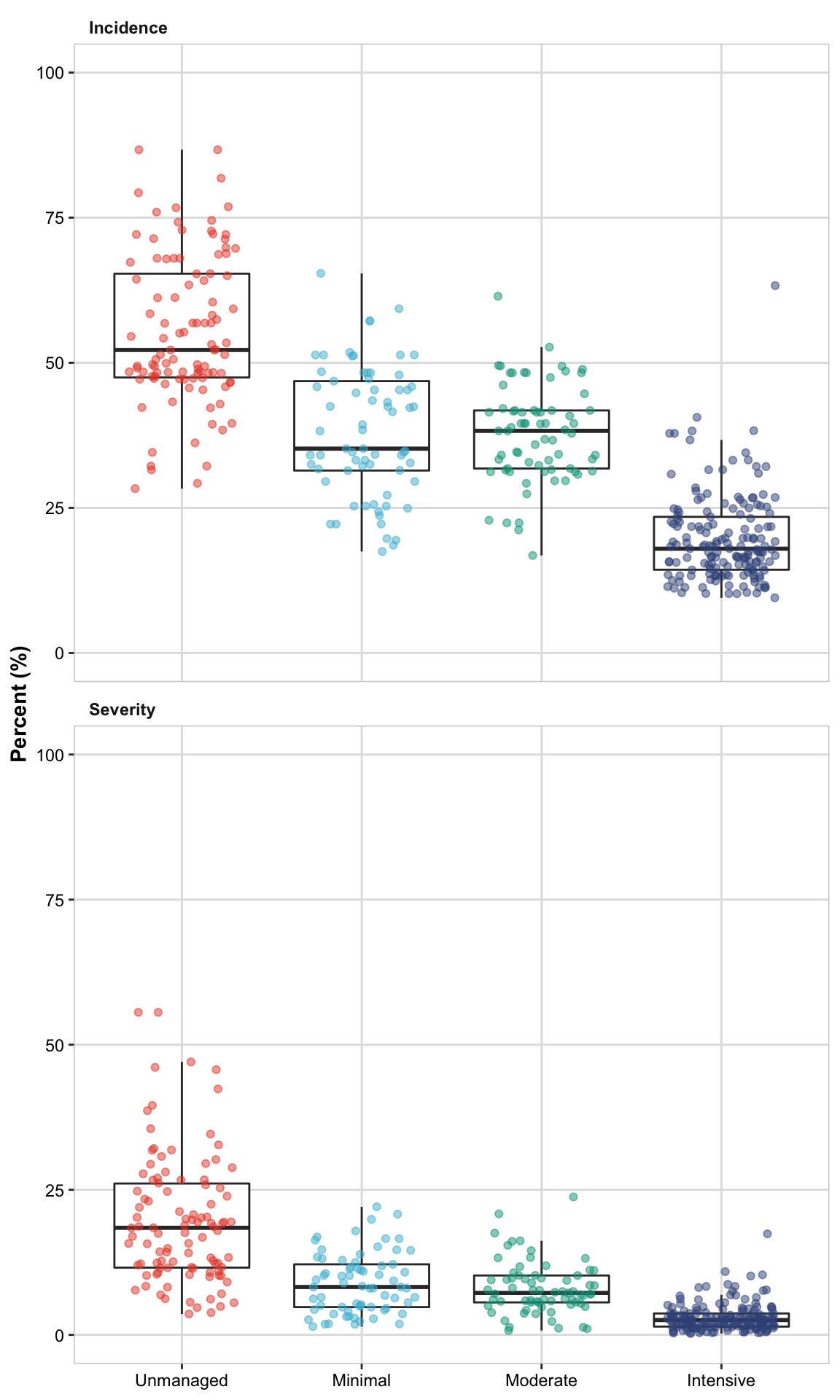 # Extra plots
Here we explore using geom_errorbar()
 demo_data =
  survey_data %>%
    group_by(farm_management) %>%
    summarise(inc_m = mean(inc),
              inc_sd = sd(inc),
              lower = inc_m-inc_sd,
              upper = inc_m+inc_sd)

  demo_data
## # A tibble: 4 x 5
## farm_management inc_m inc_sd lower upper
## * <fct> <dbl> <dbl> <dbl> <dbl>
## 1 Unmanaged 55.4 12.9 42.6 68.3
## 2 Minimal 38.0 11.1 26.9 49.2
## 3 Moderate 37.8 8.31 29.5 46.1
## 4 Intensive 19.7 7.56 12.1 27.2 ggplot(demo_data, aes(x = farm_management, y = inc_m))+
geom_errorbar(aes(ymin = lower, ymax = inc_m+inc_sd), width=.1)+
geom_point()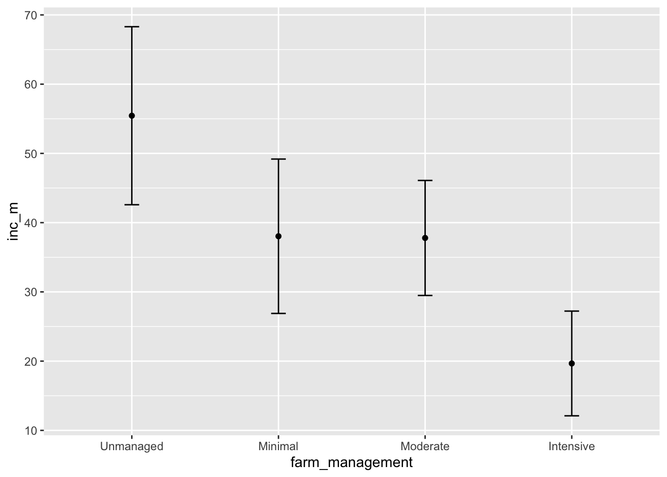
  ggplot(demo_data, aes(x = farm_management, y = inc_m))+
    geom_linerange(aes(ymin = lower, ymax = inc_m+inc_sd),
                   color = "grey", size = 2)+
    geom_point(size=2)+

    coord_flip()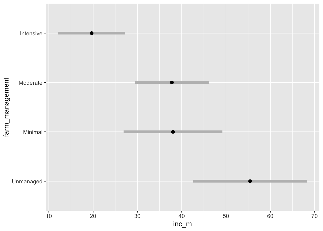
  ggplot(data = demo_data, aes(x = farm_management, y = inc_m))+

    geom_jitter(data = survey_data, aes(x = farm_management, y = inc),
                width = 0.3, alpha = 0.2)+

    geom_linerange( aes(ymin = inc_m-inc_sd, ymax = inc_m+inc_sd),
                    color = "black", size = 2, alpha = 0.6)+

    geom_point(size=4, shape = 18, color = "red") + coord_flip()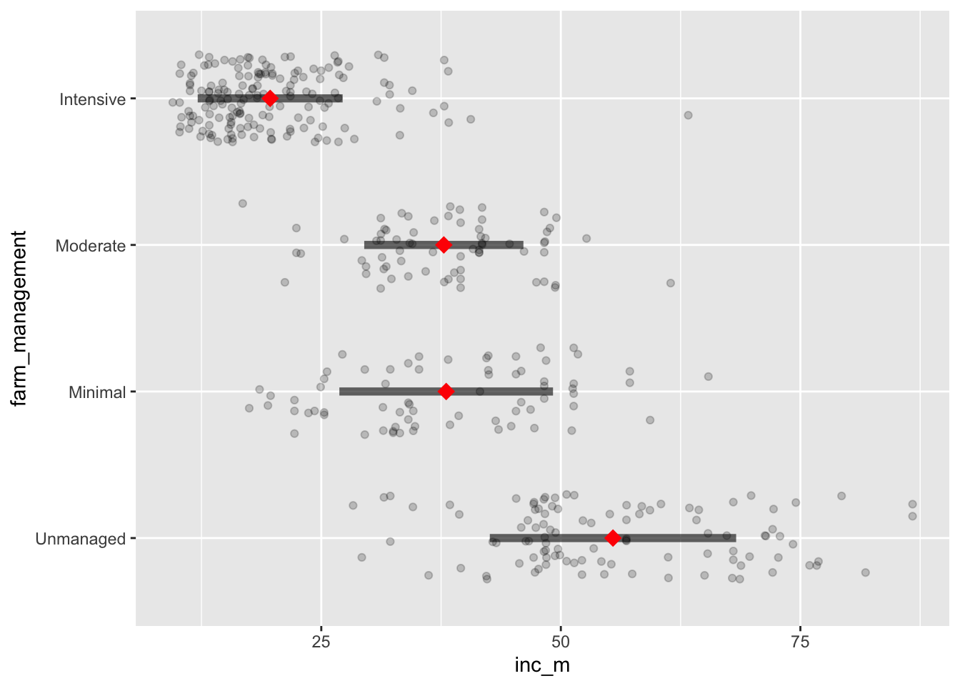
Combining multiple plots
There are several packages that can be used to combine multiple plots, one that we like is “ggpubr”.
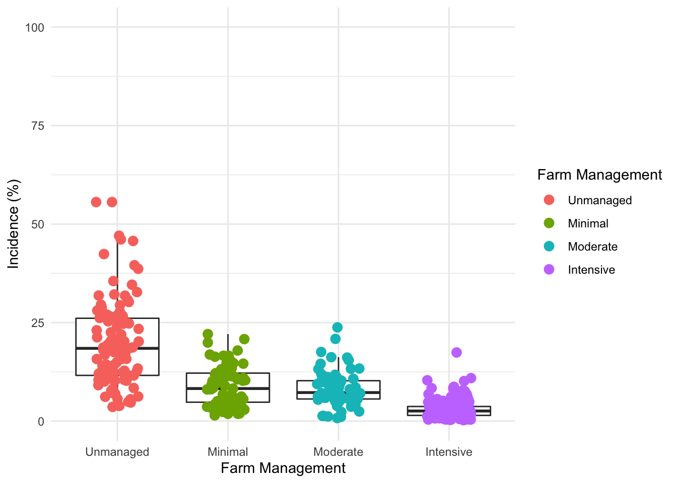
p5 = ggplot(survey_data,  aes(x= farm_management, y = inc))+
  geom_boxplot(outlier.alpha = 0) +
  geom_jitter(aes(colour = farm_management),
              width = 0.2,size = 3)+
  scale_y_continuous(name = "Incidence (%)",
                       breaks = c(0,25,50, 75, 100),
                       limits = c(0,100)) +
  labs(color='Farm Management') +
  xlab("") +
  theme_minimal()

p5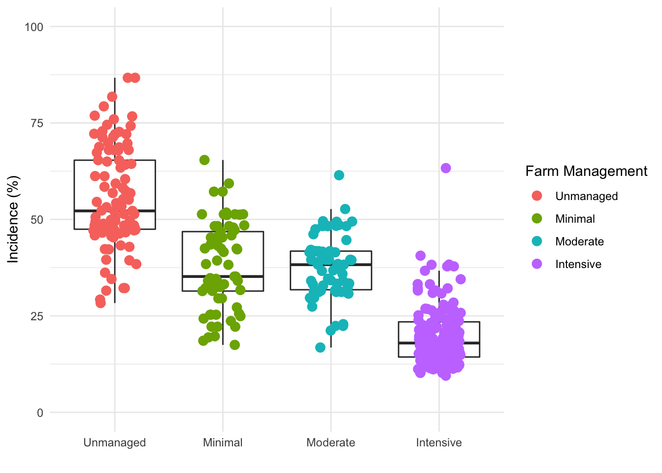
p6 = ggplot(survey_data,  aes(x= farm_management, y = sev2))+
  geom_boxplot(outlier.alpha = 0) +
  geom_jitter(aes(colour = farm_management),
              width = 0.2,size = 3) +
  scale_y_continuous(name = "Incidence (%)",
                       breaks = c(0,25,50, 75, 100),
                       limits = c(0,100)) +
  labs(color='Farm Management') +
  xlab("Farm Management") +
   theme_minimal()

p6