A simple example

Consider a simple adjacency matrix, which will be used to illustrate the functions.

library('igraph')
Amat <- matrix(c(1,0,0,0,1,1,0,0,0,1,1,0,1,1,1,1),nrow=4,ncol=4)
Amati <- graph.adjacency(Amat)
plot(Amati)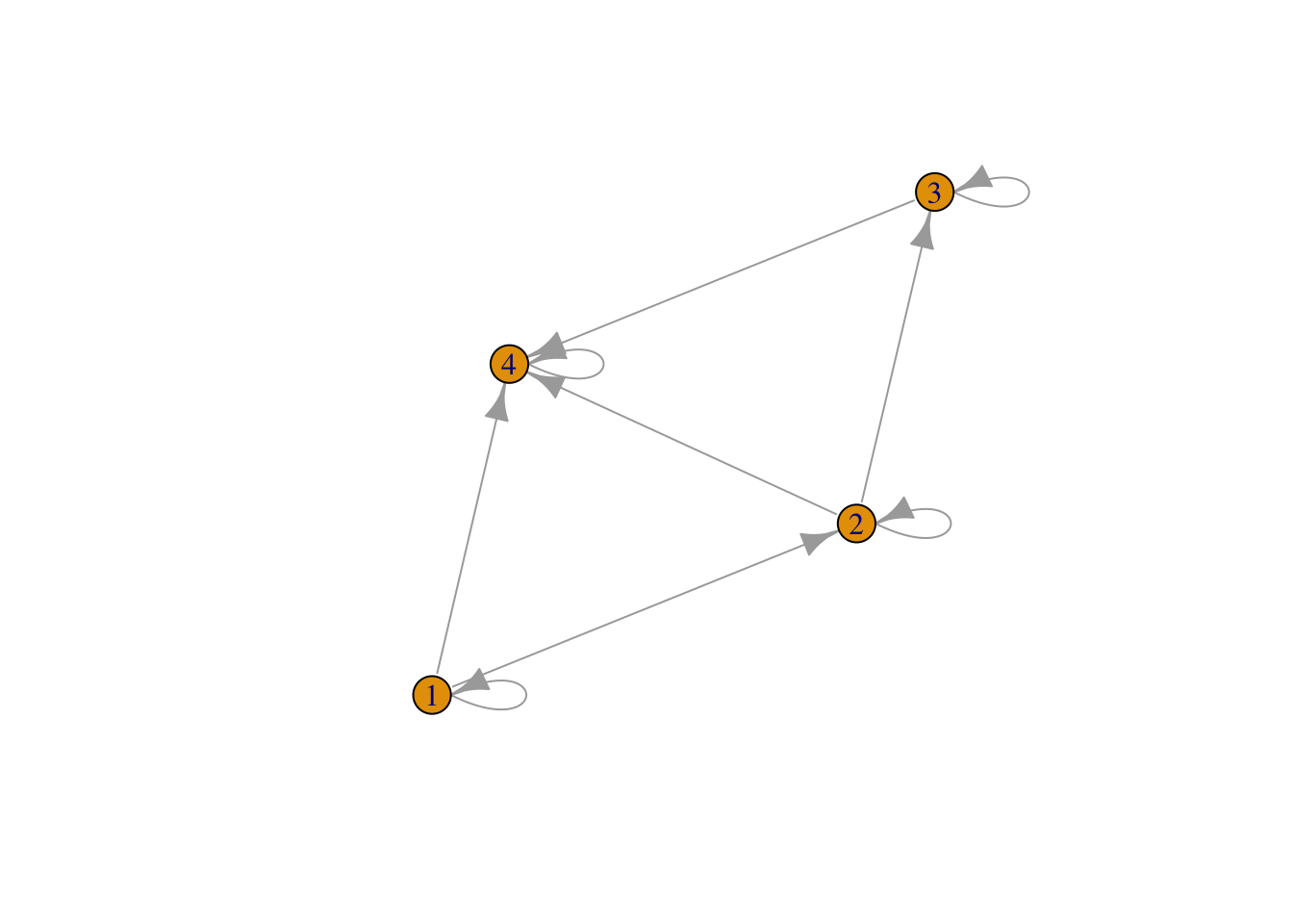

sAmat <- Amat * 0.7 # each potential link has probability 0.7 of existing - this will sometimes be useful

Illustration

For a single selected starting node, the invdetf function yields a vector of the number of nodes invaded for each sampling node by the time invasion reaches (is detected at) that sampling node, and the time step of first invasion at the sampling node - for one simulation.

The following code creates the function invdetf.

invdetf <- function(adjmat, start.choice, stoch=F){

  ### for all three functions, need to add in the definitions for the input variables...
  
  dimL <- dim(adjmat)[1] # number of rows of adjacency matrix
  t1 <- matrix( 0 * 1:dimL, nrow=1)
  t1[,start.choice] <- 1 # starting node labelled 1
  
  # if a stochastic model, generate the adjacency matrix for this simulation
    # if stochastic, assumes the adjacency matrix is made up of probabilities

  if(stoch){ # need to think about the temporal resolution of stochasticity...
    adjmat <- (matrix(runif(dimL^2), ncol=dimL) < adjmat)
  }

  # generate the infection status for each node at each time point until spread stops

  outmat <- t1
  infcount.pre <- 1
  infcount.post <- -9 # perhaps improve structure

  while(sum(t1) < dimL & infcount.pre != infcount.post){
    infcount.pre <- sum(t1) # perhaps change to infcount.pre <- infcount.post
    t1 <- as.numeric(t1 %*% adjmat > 0)
    infcount.post <- sum(t1)
    outmat <- rbind(outmat,t1) # row i is the ith time point
  }

  # find the num infected for each single sampling node, 
     # assuming infected node stays infected...
    # consider whether to set diag...

  # find the number of nodes infected at each time
  inft <- rowSums(outmat)

  # find the first time each node is invaded, and number of nodes infected at that time
  firstt <- -99 + 0*1:dimL # first time each node is invaded
  numt <- firstt # number of nodes infected at that time

  for (i in 1:dimL){ # col i is the ith sample node

    if (sum(outmat[,i] > 0)){ # if node i ever gets infected
      firstt[i] <- min(which(outmat[,i] > 0)) # first time
      numt[i] <- inft[firstt[i]] # how many nodes at that time
    }
    else {
      firstt[i] <- Inf
      numt[i] <- max(inft)
    }

  }

  # for each node, time first invaded and number of nodes infected at that time
  sampnode <- cbind(firstt, numt)

  list(outmat=outmat, sampnode=sampnode)
}

The output is two matrices. The first matrix gives the infection status for each node (column) at each time point (row) until there is no further spread. The second matrix gives, for each node (row), the time until infection (column 1) and the number of nodes infected when at that time (column 2).

invdetf(adjmat=Amat, start.choice=2) # in this case, the second node was selected as the starting point

## $outmat
##    [,1] [,2] [,3] [,4]
##       0    1    0    0
## t1    0    1    1    1
## t1    0    1    1    1
## 
## $sampnode
##      firstt numt
## [1,]    Inf    3
## [2,]      1    1
## [3,]      2    3
## [4,]      2    3

invdetf(adjmat=sAmat, start.choice=2,stoch=T) # stochastic version

## $outmat
##    [,1] [,2] [,3] [,4]
##       0    1    0    0
## t1    0    0    1    0
## 
## $sampnode
##      firstt numt
## [1,]    Inf    1
## [2,]      1    1
## [3,]      2    1
## [4,]    Inf    1

The function allstartf summarizes this analysis across all potential starting points. The following code creates allstartf.

allstartf <- function(adjmat2, stoch2=F){

  dimL <- dim(adjmat2)[1]

  alloutmat <- matrix(-99, ncol=dimL, nrow=dimL)

  for (i in 1:dimL) {
    alloutmat[i,] <- invdetf(adjmat=adjmat2, start.choice=i, stoch=stoch2)$sampnode[,2]
  }

alloutmat
}

The output is a matrix with entries being the number of nodes infected by the time an invasion is detected at each potential sampling node. Rows in this matrix are potential introduction nodes and columns are potential sampling nodes. For the stochastic case, the result is based on only one simulation (at this point in the analysis).

Note that the diagonal contains ones, because when a node is both the starting point and the sampling point, the epidemic will only have reached one node before detection.

allstartf(adjmat2=Amat)

##      [,1] [,2] [,3] [,4]
## [1,]    1    3    4    3
## [2,]    3    1    3    3
## [3,]    2    2    1    2
## [4,]    1    1    1    1

allstartf(adjmat2=sAmat, stoch2=T)

##      [,1] [,2] [,3] [,4]
## [1,]    1    3    4    3
## [2,]    3    1    3    3
## [3,]    2    2    1    2
## [4,]    1    1    1    1

The function multisimf performs the same analysis, for the specified number of simulations.

multisimf <- function(adjmat3, stoch3=F, nsim=1) {

  dimL <- dim(adjmat3)[1]

  outarr <- array(-99, c(dimL,dimL,nsim)) # all results
  meanarr <- matrix(-99, ncol=dimL, nrow=dimL) # mean of results
  vararr <- meanarr # variance of results

  for (i3 in 1:nsim){
    tempout <- allstartf(adjmat2=adjmat3,stoch2=stoch3)
    outarr[,,i3] <- tempout
  }

  for (i3 in 1:dimL) {
    for (i4 in 1:dimL) {
      meanarr[i3,i4] <- mean(outarr[i3,i4,])
      vararr[i3,i4] <- var(outarr[i3,i4,])
  } }
# consider potential use of apply to replace the second loop

  list(outarr=outarr, meanarr=meanarr, vararr=vararr)
}

The first component of the output from multisimf is the response for each simulation - nsim outputs from allstartf (in this example, 10 simulations). The next component of the output is the mean across the simulations. The final component is the variance across simulations.

Because columns represent potential sampling nodes, the mean of a column (in the second component of the output) is the mean number of nodes invaded by the time the invasion would be detected at that node. The mean of the variance in a column (in the third component of the output) indicates how consistently the mean number of nodes would have been invaded.

(AN OPTION NOT TO SHOW ALL SIMULATION RESULTS WILL BE INCLUDED)

multisimf(adjmat3=sAmat, stoch=T, nsim=10)

## $outarr
## , , 1
## 
##      [,1] [,2] [,3] [,4]
## [1,]    1    3    4    3
## [2,]    3    1    2    3
## [3,]    2    2    1    2
## [4,]    1    1    1    1
## 
## , , 2
## 
##      [,1] [,2] [,3] [,4]
## [1,]    1    3    4    3
## [2,]    2    1    2    2
## [3,]    2    2    1    2
## [4,]    1    1    1    1
## 
## , , 3
## 
##      [,1] [,2] [,3] [,4]
## [1,]    1    2    3    4
## [2,]    2    1    2    2
## [3,]    2    2    1    2
## [4,]    1    1    1    1
## 
## , , 4
## 
##      [,1] [,2] [,3] [,4]
## [1,]    1    2    3    2
## [2,]    2    1    2    2
## [3,]    2    2    1    2
## [4,]    1    1    1    1
## 
## , , 5
## 
##      [,1] [,2] [,3] [,4]
## [1,]    1    3    4    3
## [2,]    3    1    2    3
## [3,]    1    1    1    1
## [4,]    1    1    1    1
## 
## , , 6
## 
##      [,1] [,2] [,3] [,4]
## [1,]    1    2    2    2
## [2,]    3    1    3    3
## [3,]    2    2    1    2
## [4,]    1    1    1    1
## 
## , , 7
## 
##      [,1] [,2] [,3] [,4]
## [1,]    1    1    1    1
## [2,]    3    1    3    3
## [3,]    1    1    1    1
## [4,]    1    1    1    1
## 
## , , 8
## 
##      [,1] [,2] [,3] [,4]
## [1,]    1    3    4    3
## [2,]    1    1    1    1
## [3,]    2    2    1    2
## [4,]    1    1    1    1
## 
## , , 9
## 
##      [,1] [,2] [,3] [,4]
## [1,]    1    2    4    4
## [2,]    3    1    3    3
## [3,]    1    1    1    1
## [4,]    1    1    1    1
## 
## , , 10
## 
##      [,1] [,2] [,3] [,4]
## [1,]    1    3    3    3
## [2,]    3    1    3    3
## [3,]    2    2    1    2
## [4,]    1    1    1    1
## 
## 
## $meanarr
##      [,1] [,2] [,3] [,4]
## [1,]  1.0  2.4  3.2  2.8
## [2,]  2.5  1.0  2.3  2.5
## [3,]  1.7  1.7  1.0  1.7
## [4,]  1.0  1.0  1.0  1.0
## 
## $vararr
##           [,1]      [,2]      [,3]      [,4]
## [1,] 0.0000000 0.4888889 1.0666667 0.8444444
## [2,] 0.5000000 0.0000000 0.4555556 0.5000000
## [3,] 0.2333333 0.2333333 0.0000000 0.2333333
## [4,] 0.0000000 0.0000000 0.0000000 0.0000000

Weighted likelihood of a node being an entry point into network

The calculations of means up to this point have been based on the assumption that each node is equally likely to be the starting node. (Alternative functions, under preparation, do include the option for nodes to have different probabilities of invasive establishment - with suffix wt)

The function wtsimf uses output from multisimf to evaluate the mean number of nodes reached when invasion would be detected at each potential sampling node, where potential starting nodes may have different probabilities of functioning as starting nodes. For example, higher risk of being the starting node might result from a node’s role as a port, or weather conditions associated with a node.

wtsimf <- function(msf.out, adjmat5, wtvec, nodenam=NA) {

  dimL <- dim(adjmat5)[1]

  matop <- msf.out$meanarr
  wtarr <- wtvec * matop

  # find failure rate for each sampling node
  sampfail <- colSums(wtarr)
  tsampfail <- data.frame(1:dimL, sampfail, nodenam)
  
  list(wtarr=wtarr, tsampfail=tsampfail)
}

This gives the failure rate. Sometimes a more useful summary might be expressing this in terms of success rates, in the sense of the number of nodes that are not infected when the pathogen is detected by a sampling node.

Suppose the weights indicating the probability that each of four nodes is the introduction node are as follows.

wtvec.ex <- c(0.001,0.2,0.798,0.001) # weights indicating the relative likelihood that each of four nodes is the introduction node for an invasion 

msf.outex <- multisimf(adjmat3=sAmat, stoch=T, nsim=10)

wtsimf(msf.out=msf.outex, adjmat5=sAmat, wtvec=wtvec.ex)

## $wtarr
##        [,1]   [,2]   [,3]   [,4]
## [1,] 0.0010 0.0022 0.0026 0.0026
## [2,] 0.3400 0.2000 0.3400 0.3400
## [3,] 1.3566 1.3566 0.7980 1.3566
## [4,] 0.0010 0.0010 0.0010 0.0010
## 
## $tsampfail
##   X1.dimL sampfail nodenam
## 1       1   1.6986      NA
## 2       2   1.5598      NA
## 3       3   1.1416      NA
## 4       4   1.7002      NA

wtsimf(msf.out=msf.outex, adjmat5=sAmat, wtvec=wtvec.ex, nodenam=c("KS","NE","ND","SD"))

## $wtarr
##        [,1]   [,2]   [,3]   [,4]
## [1,] 0.0010 0.0022 0.0026 0.0026
## [2,] 0.3400 0.2000 0.3400 0.3400
## [3,] 1.3566 1.3566 0.7980 1.3566
## [4,] 0.0010 0.0010 0.0010 0.0010
## 
## $tsampfail
##   X1.dimL sampfail nodenam
## 1       1   1.6986      KS
## 2       2   1.5598      NE
## 3       3   1.1416      ND
## 4       4   1.7002      SD

Using the weights based on the number of information sources, or the quality of information sources, is one way to integrate the socioeconomic network and the biophysical network, with an egocentric network focus. There are many other possibilities for linking the two networks, potentially drawing on more information about the network of information communication. An example of this analysis applied to potential spread of disease through a seed system is available in

Buddenhagen, C. E., J. F. Hernandez Nopsa, K. F. Andersen, J. Andrade-Piedra, G. A. Forbes, P. Kromann, S. Thomas-Sharma, P. Useche, and K. A. Garrett. 2017. Epidemic network analysis for mitigation of invasive pathogens in seed systems: Potato in Ecuador. Phytopathology 107:1209-1218.

Andersen KF, Buddenhagen CE, Rachkara P, Gibson R, Kalule S, Phillips D, Garrett KA, 2018. Modeling epidemics in seed systems and landscapes to guide management strategies: The case of sweetpotato in Northern Uganda. Phytopathology, https://doi.org/10.1094/PHYTO-03-18-0072-R